Mobile Monitoring—Open-Source Based Optical Sensor System for Service-Oriented Turbidity and Dissolved Organic Matter Monitoring
 Robert Schima1,2*
  Stephan Krüger3 Jan Bumberger2 Mathias Paschen1 Peter Dietrich2,4 Tobias Goblirsch2
- 1Chair of Ocean Engineering, Faculty of Mechanical Engineering and Marine Technology, University of Rostock, Rostock, Germany
- 2Department of Monitoring and Exploration Technologies, UFZ - Helmholtz Centre for Environmental Research, Leipzig, Germany
- 3Chair of Soil Resources and Land Use, Institute of Soil Science and Site Ecology, Technische Universität Dresden, Tharandt, Germany
- 4Center for Applied Geoscience, Eberhard-Karls-University of Tübingen, Tübingen, Germany
The protection and sustainable use of aquatic resources require a better understanding of fresh water sources, limnic ecosystems, and oceans. The effects of global change, intensive use of natural resources and the complex interactions between humans and the environment show different effects at different scales. Current research approaches are not sufficient to appropriately take account of the heterogeneity and dynamics of aquatic ecosystems. A major challenge in applied environmental research is to extend methods for holistic monitoring and long-term observation technologies with enhanced resolution over both space and time. In this study, turbidity and the content of dissolved organic matter (DOM) are key parameters, as they are of importance for assessing the health of aquatic ecosystems and the state of ecosystem services (e.g., the provision of drinking water). Photonics and optical sensors as well as integrated circuits and open-source based components open interesting possibilities to overcome the current lack of adaptive and service-oriented sensor systems. An open source based optical sensor system was developed, which enables a user-specific, modular and adaptive in-situ monitoring of the turbidity and the dissolved organic substance content almost in real time. Quantification is based on attenuation or transmission measurements with two narrowband LEDs and corresponding detectors in the ultraviolet (DOM content) and infrared range (turbidity) of the electromagnetic spectrum. The developed in-situ sensor system shows a very high agreement with the results obtained using a laboratory photometer but with less methodological effort. First tests carried out in the area close to the city of Leipzig (Saxony, Germany) show promising results. The in-situ sensor system is able to acquire the optical attenuation with a sampling rate up to 0.1 Hz. Due to the fact that data is visualized directly with the help of web services, even the quality of data collection can be improved by assisting the selection of sampling points or a direct spatio-temporal data feedback. What this approach illustrates is the fact that open-source technologies and microelectronics can now be used to implement resilient and promising sensor systems that can set new standards in terms of performance and usability within applied environmental research.
1. Introduction
The conservation and use of aquatic resources necessitate a better understanding of freshwater sources, limnic ecosystems, and oceans to sustainably secure the livelihood of a steadily growing world population. A major challenge is seen in the fact that global change and the consequences of human action show different effects at different scales (Chapman, 1996). State of the art research approaches and scientific measurement methods are limited to large-scale measurement campaigns carried out by scientific or governmental institutions. Due to the high methodical effort and the relatively low spatio-temporal coverage, such approaches are not yet feasible enough to provide a monitoring solution to address the heterogeneity and dynamics of aquatic ecosystems in an appropriate manner (Wiemann et al., 2018).
In the field of applied environmental research, different approaches exist to measure and visualize processes in the environment and their effects on the ecosystem. These approaches extend over several scales. Starting with satellite-based earth observation, airborne, or unmanned aerial vehicles (UAVs), environmental data acquisition is also achieved by deploying sensor networks, autonomous systems, or conducting classical manual field sampling using appropriate sampling and measurement technologies for the monitoring.
What is urgently needed, however, are methods that go beyond classical established environmental research. With the help of miniaturized, integrated sensors, user groups outside science could also be integrated into the process of collecting environmental data (Citizen Science). This requires suitable sensor systems that are both easy to use and easy to process and visualize the data later on. In current research, there are approaches that investigate new strategies of environmental data collection with a similar motivation (Hut et al., 2016; Brewin et al., 2017; Seibert et al., 2019). It is particularly important to develop approaches for a wide range of users when determining, controlling and ensuring good water quality in the long term (Lockridge et al., 2016). Under these aspects, an efficient sensor system must not only provide scientifically valid data. For the later utilization of the data, appropriate interfaces must be created for visualization, online availability of the data and for the creation of a spatial reference for measurement (e.g., via GPS).
Therefore, this paper presents and evaluates an approach for such a monitoring based on an optical measuring system for the determination of dissolved organic carbon and turbidity.
1.1. Water Quality Assessment
Especially with regard to the process dynamics and heterogeneity of aquatic ecosystems, a comprehensive monitoring of these effects remains to be a challenging issue. This results in a strong pull to develop adaptive survey and monitoring strategies as well as tools to observe even complex ecosystems of large scale and over a longer period of time. In this connection, it is of particular interest to map the heterogeneity as well as the dynamics of processes in a discrete manner to address the spatio-temporal interdependencies of aquatic systems appropriately. Although the performance of sensors and sensor systems has considerably increased during the last years, the integration of data as well as the provision of gathered information have to be improved to achieve a more wide spread use of optical sensors and sensor systems in practice. In terms of optical tools for aquatic monitoring a broad review is given by Moore et al. (2009). The motivation of this work is the development and implementation of an in-situ sensor probe prototype for the optical detection of dissolved organic carbon (DOC) in aquatic media.
1.1.1. Dissolved Organic Carbon (DOC)
Dissolved organic carbon is a sum parameter and represents all organic compounds dissolved in water. It plays a key role in the assessment of water status and load (Guo et al., 1995). In the field of water and environmental research, the interest in observing and documenting short and long-term trends in DOC concentrations of surface and drinking water is of great importance (Kolka et al., 2008). Current field devices for the recording of DOC are very reduced with regard to their modifiability by the user and are not designed for near real-time data processing. Another limitation of current system is the insufficient temporal-spatial resolution. The implementation of mobile monitoring strategies is therefore difficult to achieve.
1.1.2. Turbidity
Turbidity describes how clear a selected volume of water is. In this context, turbidity refers to the presence of suspended solids. The more turbid a water is, the less light can be transmitted through it as a result of the suspended solids. With regard to ecosystem processes, increased turbidity means, for example, that less light is available for photosynthesis (Bass et al., 1995). The interaction therefore has an effect on aquatic fauna, but also on fish abundance and distribution. Furthermore, turbidity is often related to the nutrient content, which strongly influences an ecosystem (Chapman, 1996). In addition to the ecological aspects, turbidity is of great importance as a corrective in applied measurement techniques. Knowledge of turbidity is important to enable appropriate corrective measures when working with optical instruments in general (turbidity correction).
1.2. Sensing as a Service
To this end, an open-source based, modifiable in-situ probe would represent a promising possibility to realize a mobile and cross-scale monitoring approach, which allows a higher spatial and temporal resolution with lower maintenance and acquisition costs. For this purpose this work aims at the proof of concept and the development of an optical sensor probe as part of a sensor system for the detection of DOC under field conditions based on a spectrometric measurement.
As another aspect of this work, it will be investigated to what extent cost-effective open-source based platforms are suitable for realizing complex environmental information and sensor systems. Raspberry Pi, Arduino and other technological developments, especially in the field of IoT and miniaturized automation, have fundamentally changed the working methods of different user groups and the way inventions can be realized with very limited resources.
In addition to the construction of a field-capable sensor unit, the development of powerful and fast data processing structures is another motivation of this work in order to provide reliable monitoring data close to real-time. To achieve this goal web based services were developed and implemented. In this connection, the definition of standards as well as the establishment of suitable interfaces were key elements to create an holistic process chain from the acquisition of a single measurement to the provision of reliable information for decision making, which is called Sensing as a Service.
In contrast to common monitoring approaches using stationary observation data, mobile monitoring approaches provide the potential of a higher spatial resolution in terms of identifying the heterogeneity of an ecosystem. For a service-oriented implementation of the necessary computation, especially during the field measurements, an abstract data model was formulated called the Object Specific Exposure (OSE) (Schima et al., 2017; Schima, 2018). The term exposure is used to describe the relationship between a state variable, e.g. the measured concentration of organically dissolved carbon, and the respective period or reference space of the measurement. A mobile measurement series along a river section must therefore be interpreted differently than a stationary measurement in the same period. A simple averaging, however, is not sufficient, since the integral information contained with regard to the temporal and spatial peculiarities would be lost. This approach serves as a holistic representation of an exposure, e.g., an object exposed to a concentration (c) of a substance at a specific position (x, y), at a specific depth (z) and for a specific amount of time (t) in an aqueous media as shown in Equation (1).
In view of mobile sampling, it is necessary to establish a corresponding spatial and temporal reference for each measurement of a state variable [e.g., concentration (c)]. The exposure is then composed integrally (see Equation 1). The OSE formula is a considerable help for the development of mobile sensors since applied as a design and system paradigm, it ensures that all descriptive data of a measurement conversion is generated at the sensor level. The optical in-situ measurement of absorption is thus supplemented by information such as location, water depth, time, and system status. Furthermore, a strict monitoring paradigm ensures that, for example, a measured value is only collected at full minute intervals. This allows the direct comparison of data from different sensor systems with no need for any further data harmonization.
At the same time, the usability of the collected data is increased. Following the OSE paradigm and using standardized interfaces for data transmission, real-time environmental information systems can be set up. This makes it possible, for example, to create a map display in the field while collecting the data or to visualize time series on a smartphone or tablet. The joint development of hardware and software leads to a so-called Assisted Monitoring, which is particularly useful for mobile applications as shown in the following.
1.2.1. Assisted Monitoring: Mobile App and Web Service
The approach of an Assisted Monitoring aims at providing the user with reliable information on the target environmental parameters and sensor system states during data collection (see Figure 1A). To do so, the system consists of an optical sensor head that is connected to a control and communication unit. Via a Bluetooth interface it is possible to configure the measuring system with the help of a mobile terminal device and an app (see Figure 1B), to start measurements manually or automatically and to send the measured values via a web interface, e.g., for online visualization (see Figure 1C).
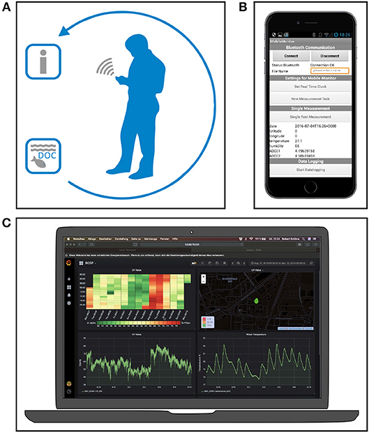
Figure 1. Assisted Monitoring based on mobile apps and web services will lead to new perspectives in environmental monitoring and observation. The development of service-oriented infrastructures will accelerate the data acquisition toward the provision of reliable information during field measurements (A). The visualization of data near real-time and the usage of mobile devices (B) in the field will increase the spatio-temporal resolution and the quality of environmental monitoring in general (C).
The mobile app empowers the user to modify the data acquisition and to configure the sensor system. Therefore, single measurements or an automated monitoring can be easily achieved. The app provides an initial data evaluation and a real-time data visualization. During the measurement, data can be stored locally or send to a web service.
On the server side, various services take over the forwarding, processing and visualization of the data. A browser based web service provides a dashboard for real-time data visualization including a web map service for initial interpretation of the data, e.g., in the field for ad-hoc adjustments of the sampling strategy. Here again, the sensor system development according to the OSE paradigm allows a straight data stream processing since every single measurement is geo referenced and time synchronized. The data stream process requires the following process stack per each measurement:
1. Sensor level:
(a) Routine to acquire all data from the sensor system (e.g., temperature, pressure, absorption,…)
(b) Routine to generate a message string containing all predefined values of interest
(c) Routine to configure communication module according to the used communication protocol
2. Sensor level:
(a) Message-oriented middleware (MOM) – A message broker to handle the incoming messages, e.g., RabbitMQ
(b) A data base to store the data, e.g., InfluxDB
(c) A front end to query and visualize the data, e.g., Grafana
In order to feed conventional environmental data processing, a data export function can be used to export the data in an appropriate format, e.g., as a comma separated values file.
2. Materials and Methods
2.1. Measurement Principle
The underlying measuring principle is an optical transmission measurement (respectively attenuation) of water due to different ingredients and dilutes (Preisendorfer, 1976; Bass et al., 1995; Hoge et al., 1995). This measuring principle is well-established in laboratory analysis, so that regulations exist for the detection of certain substances in water. To comply with normed methods and standards, the use of DIN standards is common in Germany. DIN (Deutsches Institut für Normung) is the German Institute of standards. The relevant standards for this study are the DIN 38404-3 (2005) for attenuation in the UV wavelength range, DIN EN 1484 (1997) for DOC analysis and DIN EN ISO 7027 (2000) for turbidity approximation.
With respect to DIN 38404-3 (2005) the spectral absorption coefficient αλ or rather the Extinction Eλ at λ = 254 nm is used as a summarizing method for the determination of dissolved organic carbon in aquatic media. Therefore, the attenuation of UV light passing through a sample is detected by absorption. This measured absorbance of the water sample serves as a measure of the concentration of chromophorically dissolved organic substances in water, such as DOC. The general basis for such quantitative absorption measurement is the Beer-Lambert law according to Equation (2):
Here, Eλ represents the Extinction, I0 the intensity of emitted light in W m-2, I1 the intensity of transmitted light in W m-2, ϵλ the extinction coefficient in m2 mol-1, c the concentration of absorbing material in mol l-1 or km m-3, and d the path length in m. Based on this considerations, the development of an optical in-situ sensor probe for measuring the attenuation will be described in the following.
2.2. Hardware Description
2.2.1. Sensor Probe
According to DIN 38404-3 (2005) the spectral absorption coefficient αλ at λ = 254 nm can be used to calculate the DOC content in aquatic media. Therefore, the probe consists of an ultraviolet light emitting diode (UV-LED) as emitter and a UV photodiode as detector. Since it is not possible to filter the medium in an in-situ measurement as recommended by DIN EN 1484 (1997), for an in-situ measurement of DOC the influencing turbidity must be compensated or determined. As shown in Huang et al. (1992) and Liu and Dasgupta (1994), a spectrometric measurement at λ = 860 nm can be used to compensate the turbidity.
Dual wavelength measurement is implemented with two sensor units, a UV sensor unit for measuring DOC at λ = 254 nm and an infrared (IR) sensor unit for measuring turbidity at λ = 860 nm. To perform the photometric measurement, each sensor unit includes an emitter and detector as shown in Figure 2A. An UV-LED (UVTOP250-BL-TO18 from ROITHNER LASERTECHNIK GmbH, Vienna, Austria) (λmax = 254 nm) is installed on the emitter side of the UV unit. An IR LED (SFH 4557 from OSRAM Opto Semiconductors GmbH, Regensburg, Germany) (λmax = 850 nm) is installed for the emitting IR unit. In addition, the IR emitting sensor head includes a constant current source at ILED = 100 mA and a voltage regulator. The UV emitting sensor head contains a constant current source at ILED = 20 mA. The detector for the UV sensor unit is a UV silicon carbide photodiode (SIC01S-C18 from ROITHNER LASERTECHNIK GmbH, Vienna, Austria) with peak spectral sensitivity at λ = 254 nm. An IR LED (SFH 4850 E7800 from OSRAM Opto Semiconductors GmbH, Regensburg, Germany) is used as a detector for the IR channel. Both detector heads also include a 16-bit analog-to-digital converter (ADS1115 from Texas Instruments Incorporated, Dallas, USA). In addition, the UV receive sensor head contains a single supply instrumentation amplifier. For controlling the system, a Raspberry Pi is used. A transistor and an optocoupler are installed for each channel to control the UV LED and IR LED. A Python script running on the Raspberry Pi is responsible for managing the switching characteristics and measurement. The emitter and detector sensor heads are connected to the control unit via 4-pole cable (LifYDY 4 x 0.10 qmm of kabeltronik Arthur Volland GmbH, Denkendorf, Germany). The entire system is supplied by a battery pack (see Figure 2). With one battery charge, data can be recorded for up to 24 h. For later application the sensors are placed inside the media. The control unit (topside unit) is designed to ensure user interaction via Bluetooth, GPS positioning and data transmission via WiFi.
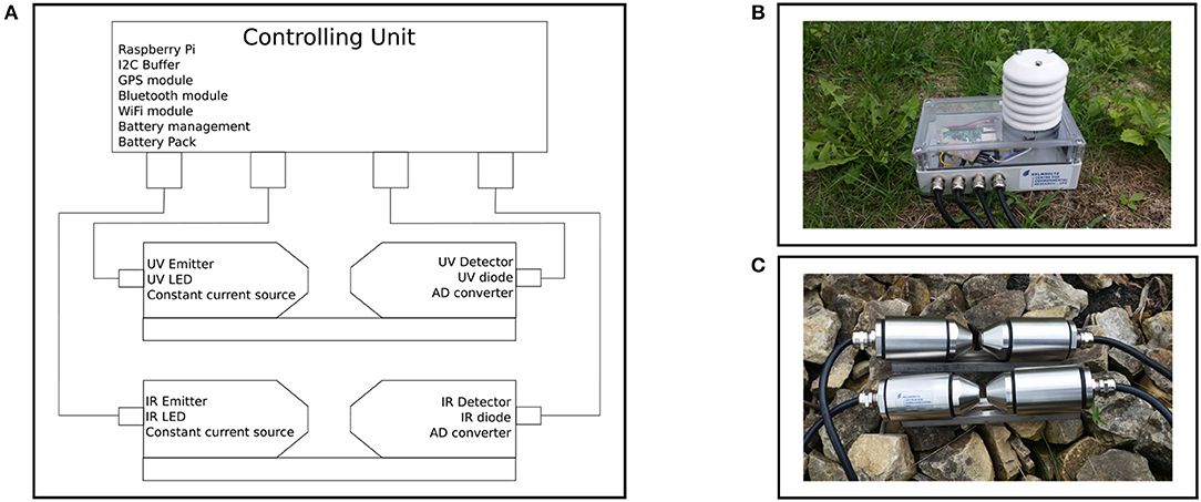
Figure 2. (A) shows a schematic drawing of the sensor system. (B) shows the control unit with the Raspberry Pi, GPS receiver, and WiFi module as well as the battery pack. Four cables are connected to the emitters and detector units of the UV channel (DOM) and IR channel (turbidity); the white attachment on the top of the control unit is used to measure temperature and humidity. The illustration in (C) shows the IR sensor unit at the top and the UV sensor unit at the bottom, with both receiving and transmitting sensor heads mounted opposite each other on a metal guide. Inside there is an LED as emitter and a photodiode as detector in combination with an AD-converter. A constant current source and voltage regulator are integrated on the emitter side for stable operation. The control unit and the sensor modules are connected by cables.
The housing of the probe is made of stainless steel. The system consists of two cylindrical sensor heads, one for the emitter and one for the detector. Both are mounted opposite of each other on a connecting bridge. Each sensor head has a sapphire glass window at the narrow end of the cylinder. The wide ends of the heads have a waterproof cable gland. Including the cable gland, the sensor measures a height of 4.4 cm, a length of 20.8 cm and a width of 3.9 cm, and weighs 119.2 g (see Figure 2C). The Python script running on the Raspberry Pi controls the time, duration, and iteration of the measurement. Both, the UV and IR units are activated simultaneously. Accordingly, as soon as the LED is supplied with power, it begins to emit light that goes through the medium and hits the detector (diode). Due to the relationship between the concentration of the measured compounds and the intensity of the transmitted light, the light intensity incident on the receiving diode varies (cf. Lambert-Beer law). In the photo diode, the incident light generates a current dependent on the intensity of the light, so that the voltage can be measured via a trans-impedance amplifier. This voltage is converted into a digital signal by the analog-to-digital converter and evaluated by the control unit (Raspberry Pi). Once the DOC and turbidity units are calibrated, the turbidity and consequently the content of DOC can be determined based on the transmission measurement.
2.3. Laboratory Experiments
2.3.1. Sensor Calibration
Both sensor units are calibrated directly in the medium. Potassium hydrogen phthalate as recommended in DIN EN 1484 (1997) is used to prepare a dilution series for DOC calibration. Even though formazine is the standard solution for the calibration of turbidity probes according to DIN EN 1484 (1997), the use of formazine is avoided due to its toxic properties. Liu and Dasgupta (1994) used milk in their experiments to produce turbidity. Since milk is an organic product, it influences the DOC measurement and therefore cannot be used for this experimental set-up. Clifford et al. (1995) used the inorganic component Fuller's Earth. Besides milk, Fuller's Earth is unsuitable due to its adsorption properties, which can lead to complications with potassium hydrogen phthalate. Talcum powder (Talcum Powder -350 MESH from Sigma-Aldrich Co. LLC., St. Louis, USA) (Mg3Si4O10(OH)2) is used as a non-adsorbent, inorganic, non-water-soluble material that does not influence the DOC measurement, in order to cause turbidity in this experimental setup. To find out how the turbidity and DOC measurement units react to different concentrations, both are mounted upside down with the receiving diode on top in a glass vessel to avoid the influence of stray light during measurement. To avoid mutual interference between the two sensor units, each sensor is inserted into the calibration vessel separately.
To prepare the dilution series, distilled water with a content of total organic carbon (TOC) of c = 0.003 mg l−1 is used as the base medium for calibration. A glass vessel is filled with V = 0.8 l distilled water. Due to this low TOC concentration, no filtering of the distilled water is required. It is intended to measure DOC concentrations of cDOC = 0, 5, 15, 25, 50, 75, 100 mg l-1. Therefore, a stock solution is prepared with c = 1000 mg l−1 potassium hydrogen phthalate. To produce the intended DOC concentrations, the following amount of stock solution is added to the V = 0.8 l zero solution (see Table 1).
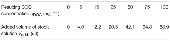
Table 1. Volume of stock solution added to V = 0.8 l zero solution to produce several DOC concentrations.
In order to be able to measure turbidity in a comparable way, formazine has become established as the turbidity standard liquid in laboratory analysis. There are different turbidity units, all of which refer to dilutions of this turbidity standard liquid, but some of which reflect different phenomena. This study refers to the turbidity unit FAU (Formazine Attenuation Units), since a transmitted light measurement, as defined in DIN EN ISO 7027 (2000), is carried out to determine this unit. Since this is the same measuring arrangement as in the present sensor design, the greatest comparability is given here. For each DOC concentration, five turbidity levels of 0, 20, 40, 60, 80 FAU are generated. To calculate the amount of talcum powder needed to produce the different turbidity levels, several concentrations of talcum powder and distilled water are produced and measured with a laboratory photometer (Spektralfotometer CADAS 50s from Hach Lange GmbH, Berlin, Germany). This results in a linear function of the talcum powder concentration and the resulting turbidity unit. Consequently, the following quantities of talcum powder are added to gradually increase turbidity from 0 to 80 FAU. Since different amounts of stock solution are added at each DOC concentration, the amount of talcum powder added varies depending on the total volume of the sample to be generated.
The measurements are performed by starting a Python script. In this study the measurement duration is tm = 10 s. With a measurement interval of ti = 0.25 s, 40 single point measurements are performed. For the IR channel, an interruption of td = 30 s is set between the turbidity measurements to avoid drifting of the turbidity sensor due to heating.
The experimental procedure is as follows. First, a sample with the required DOC concentration is prepared and thoroughly mixed. Even if a magnetic stirrer is used, it is recommended to stir the sample occasionally by hand with a glass stirrer to keep the sample homogeneous. Shortly after stirring, a small amount of the sample is taken with a pipette and placed in a quartz cuvette. The sample is shaken thoroughly five times, the turbidity is measured with the laboratory photometer and the values averaged. The sample is then mixed again by hand in the glass vessel, the IR sensor is mounted inside and the measurement is carried out. Shortly after the IR sensor has been removed, the sample is thoroughly mixed, the UV sensor is placed inside and a measurement is performed. Then the sapphire glass window of the sensor head is cleaned, the next turbidity level is prepared and the procedure is repeated for all turbidity conditions. After measuring all turbidity conditions for one DOC concentration, the entire probe is cleaned, a new sample is prepared with the required DOC concentration and the process starts again. As a result, the voltage output from the IR and DOC sensors is measured for each combination of DOC concentration and turbidity. The results and measured values of the calibration are listed in the form of tables in the Supplementary Material of this article.
For IR and UV sensor evaluation, linear regression is performed using the least squares method and the coefficients of determination. For this purpose, the sensor signals are examined with regard to the correlation to the DOC concentration for all turbidity levels. Subsequently, a multiple linear regression according to the least squares method is performed by statistical software (IBM SPSS Statistics Version 21.0.0.0.0). Since the transmission has an exponential relationship, the extinction E (cf. Lambert-Beer law) of the detector signal is used for the comparison according to Skrabal (2009). The dependent variable is the extinction of the UV sensor unit EUV, the independent variables are the DOC concentration and the turbidity. To increase the linear relationship between dependent and independent variables, the calibration data set is revised. Therefore, all calibration points near the zero signal are eliminated, in this case all points with EUV ≥ 0.164. Only the revised data set is used for the evaluation due to the fact that all other calibration points are outside the linear range.
For the revised data set, a statistical, software-based linear regression analysis is performed using the least squares method. The resulting calibration curves are determined with respect to their coefficients of determination. Linear equations are calculated for the following relationships:
Linear relationship of the IR detector signal EIR as dependent variable and the turbidity values cFAU in FAU as independent variable. m1 in FAU−1 and n1 are constants. Therefore, all calibration points are included (see Equation 3).
Regarding the linear relationship of the UV detector signal EUV(cDOC) as dependent variable and the DOC concentration cDOC in mg l-1 as independent variable, only calibration points with turbidity cFAU = 0 FAU are included (see Equation 4). m2 in l mg-1 and n2 are constants.
For the linear relationship of the UV detector signal EUV as dependent variable and the turbidity values cFAU in FAU as independent variable, only calibration points with cDOC = 0 mg l−1 are included (see Equation 5). m3 in FAU−1 and n3 are constants.
2.3.2. Turbidity Compensation
In order to be able to distinguish between the extinction as a result of turbidity and DOC content in the field, it is necessary to determine a suitable turbidity compensation method.
A practical approach is to calculate additional calibration curves by linear regression using the least squares method. The linear relationship between the UV detector signal EUV(cDOC) as a dependent variable and the DOC concentration cDOC as an independent variable for each turbidity value of the calibration data set. In addition to Equation (4) there are further linear functions for cFAU = 20 FAU, cFAU = 40 FAU, and cFAU = 60 FAU. Turbidity values greater than 80 FAU are not included in the revised calibration data set because they are outside the measurable range. After the turbidity value has been measured by the IR sensor unit, it is checked which calibrated turbidity value is closest. The corresponding calibration curve is used to calculate the compensated DOC value. All negative DOC Values are set to zero. Using the calibration points, compensated DOC values can now be calculated. Two more turbidity compensation methods are described in the Supplementary Material. However, they provide qualitatively inferior results, which is why they will not be discussed further here.
2.4. Field Measurements
The overall objective of this work is to provide an instrument for service-oriented in-situ monitoring. For this purpose, the basic feasibility will be demonstrated by means of a case study on site. To this end, two exemplary monitoring campaigns were carried out in the summer of 2016 in the urban area of Leipzig, Saxony, Germany at Lake Cospuden (see Figure 3A) and along the Elstermühlgraben, Pleiße and Elster watercourses (see Figure 3B). Lake Cospuden is an artificial lake located south of Leipzig, Saxony, Germany. It is originated from a residual mining pit that was flooded. During re-cultivation, a recreational area with beach and landscape park was created around the lake. Due to the intensive use for local recreation, the ecological condition of the lake is also of interest. For this reason, two measurement campaigns were undertaken in summer 2016 by using a small boat to investigate the situation regarding the turbidity and DOC content.
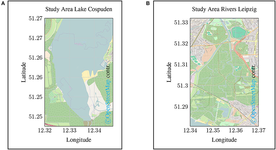
Figure 3. Map of the study areas sampled in the case study. (A) shows the opencast mining lake Cospuden in the south of Leipzig. (B) shows the course of the Elstermühlgraben, a section of the Pleiße up to its confluence with the Elster near Leipzig.
Due to the service-oriented system architecture, the methodological effort during the field measurements is moderate. As described above, the sensor system consists of the sensor probe, which is connected to the topside unit via a cable and a connector.
The controlling unit can be accessed via a USB connection or via the power supply 12 V…32 V (DC). In the present case, a USB Power Bank (TL-PB20100, Portable Power Station, 20 100 mA h. Capacity, TP-Link Technologies Co., Ltd., USA) with a capacity of 20 100 mA h was used. Thus, the measuring system can be operated for ~48 h. The sensor probe can be easily mounted using the metal brackets integrated in the sensor housing at the top and bottom.
The user thus has the option of simply placing the sensor in the water on the cable, attaching it with a rope or attaching the sensor to a device carrier or frame. Conventional measuring systems are usually larger and heavier than the sensor system presented here. With the sensor system it is therefore possible to introduce new strategies and technologies for data acquisition in addition to classical monitoring through the use of research vessels.
As a proof of concept, two monitoring campaigns were carried out within the framework of the case study. For this purpose, a monitoring with a canoe was carried out, which enables data acquisition in very shallow river basins and small streams. The sensor installation for this case is shown in Figure 4. The sensor probe is attached to a bracket that allows the depth and orientation of the sensor to be changed from on-board.
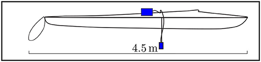
Figure 4. Sensor installation on a canoe for mobile monitoring. The canoe is 4.50 m long. The sensor was positioned in the middle of the canoe at a depth of 0.35 m below the water surface. For user-friendly handling of the sensor, it is important that it can be installed quickly and easily. Due to the low weight, the installation can be adapted to the respective installation situation.
After mounting the sensor probe, the system can be switched on without further user interaction. As long as a stable Internet connection exists, e.g., via an access point provided by a mobile phone, the data collected by the system is automatically transferred to the server and processed to a real-time data visualization via standardized web services. This is achieved with the help of the standardized data format JSON, which enables direct post-processing with the help of appropriate libraries and plug-ins.
The measurement system also works without an Internet connection and stores the data on an SD card. This prevents any loss of data as a result of a missing Internet connection.
3. Results
3.1. Calibration of the Sensor
By calibrating the IR sensor unit, the signal was determined for all DOC concentrations and the corresponding turbidity values. For all measurement series, the coefficients of determination for the linear regression of the measurement signal by the IR sensor and the measured turbidity by the laboratory photometer are significantly higher than R2 = 0.9. Consequently, there is a strong linear correlation between the decrease of the IR detector signal and the respective turbidity. Even with turbidity values greater than 80 FAU, with U ≈ 920 mV the sensor unit is not yet in the detection limit range (zero level at U ≈ 21 mV as shown in Figure 5).
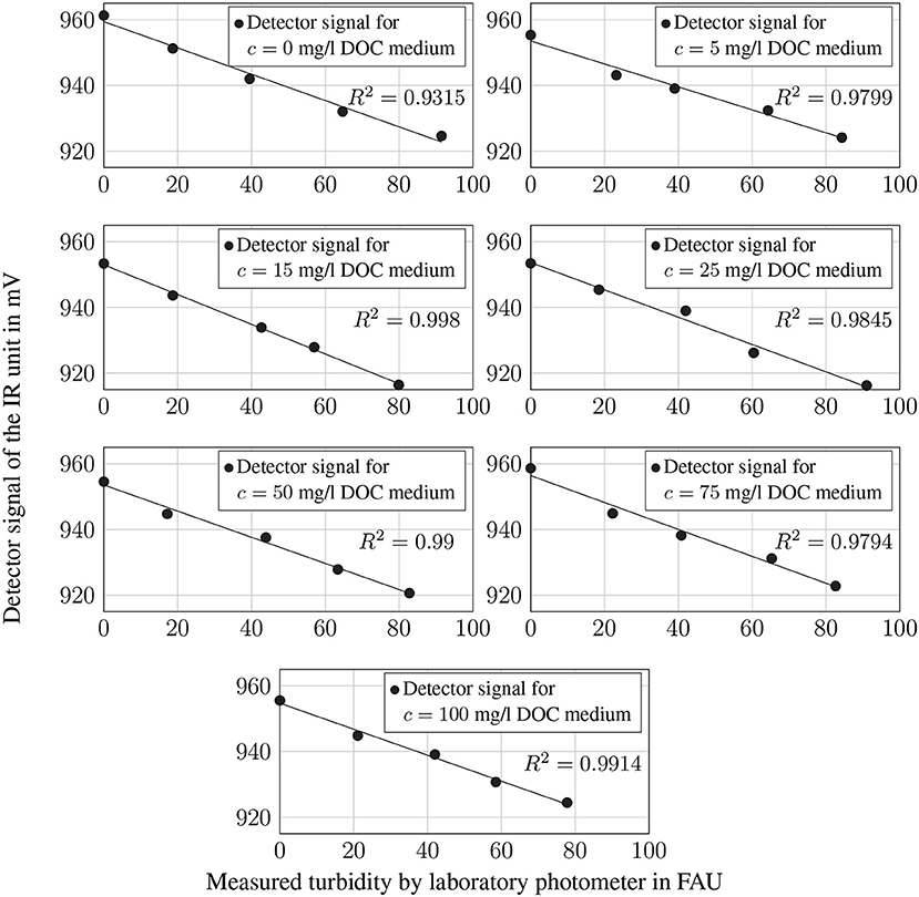
Figure 5. Measured detector signal of the IR sensor in mV for all DOC concentrations and different turbidity values in comparison with the turbidity values measured using a laboratory photometer. The trend line was generated by linear regression.
To ensure that a changing DOC concentration has no effect on the IR detector signal, it is useful to perform correlation analysis for both channels. The results for the IR detector are shown in Table 2 indicating that there is no correlation between the DOC concentration and the IR sensor signal.
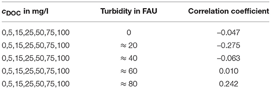
Table 2. Correlation coefficients between the IR sensor signals and the different DOC concentrations for every turbidity value.
The calibration of the UV sensor unit measures the signal for all DOC concentrations and several turbidity levels, as well as the IR sensor unit. For DOC concentrations at cDOC = 0 mg l−1, cDOC = 5 mg l−1, and cDOC = 75 mg l−1, the scale of determination of the sensor signal and turbidity is relatively high at R2 ≥ 0.9. While the measured signals correlate with R2 ≈ 0.8 at DOC concentrations of cDOC = 15 mg l−1, cDOC = 25 mg l−1, and cDOC = 50 mg l−1, the signal does not correlate with the turbidity level at cDOC = 100 mg l−1. Consequently, there is a strong linear correlation between the sensor and the turbidity caused at low DOC concentrations, which decreases with increasing turbidity. In all cases, the measured signal shows a less pronounced linearity for values close to the zero level U ≈ 3.050 mV (see Figure 6).
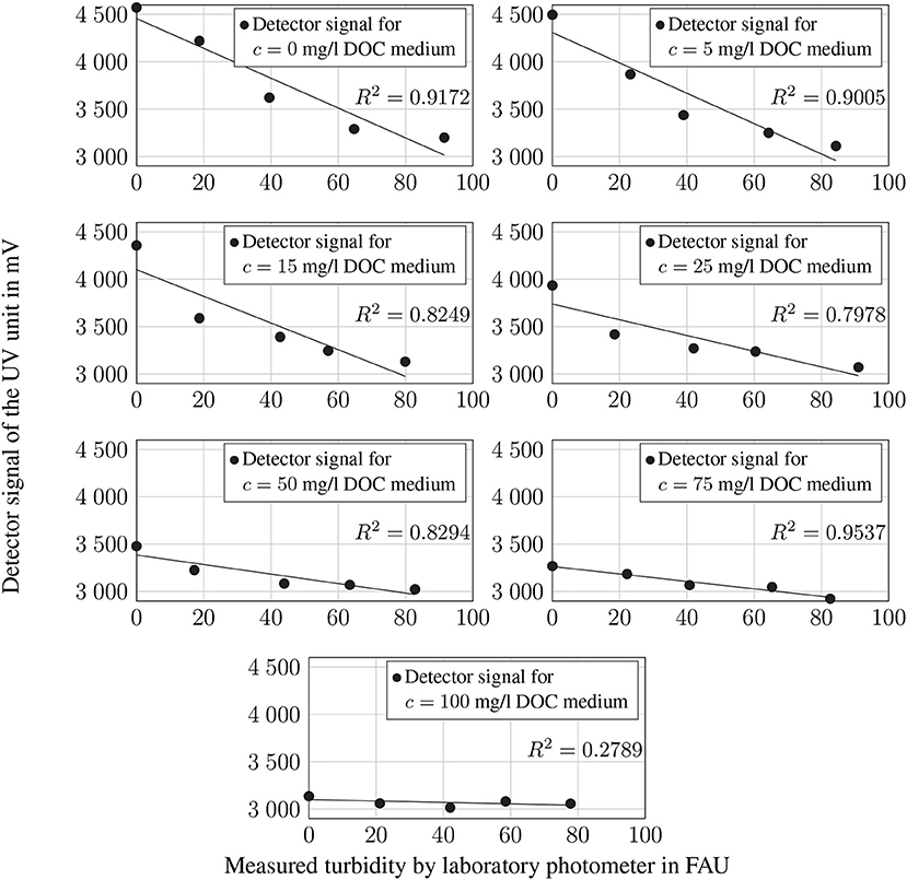
Figure 6. Measured detector signals of the UV sensor in mV for all DOC concentrations and different turbidity values in comparison to the values determined by laboratory photometers. The trend line was generated by linear regression.
In contrast to the correlation between the IR sensor signal and the DOC concentration, the UV sensor signal correlates strongly with the DOC concentration. With correlation coefficients between −0.88 and −0.97 for the first four turbidity levels, the sensor shows a strong linear correlation with the DOC concentration at low turbidity values. Only for turbidity around 80 FAU the correlation coefficient decreases in magnitude so that the relationship between the sensor signal and the DOC concentration is less pronounced (see Table 3).
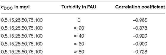
Table 3. Correlation coefficients between the UV sensor signals and the different DOC concentrations and the corresponding turbidity values.
The extinction EUV estimated by the UV sensor unit, is to be compared in the following with the DOC concentration cDOC and the respective turbidity cFAU. As shown in Figure 7, only low extinctions EUV show a linear relationship. The higher the extinction EUV, the flatter the curve. All calibration points in the blue area of the diagram are close to the zero signal. A linear relationship between the absorbance and the DOC concentration is only given for samples without turbid material. For turbidities of 20 FAU, only the cDOC ≤ 80 mg l−1 range can be described as linear. If the turbidity value rises to 60 FAU, only cDOC ≤ 25 mg l−1 can be assigned to the linear range. At 80 FAU the gradient becomes so flat that a linear relationship is no longer given (see Figure 7). Therefore, the adjusted calibration plot contains 22 of the original 35 calibration points. Compared to the unadjusted calibration data, R2 has increased from 0.765 to 0.872. Thus, the linear relationship between cDOC, cFAU and EUV has also increased (see Figure 8).
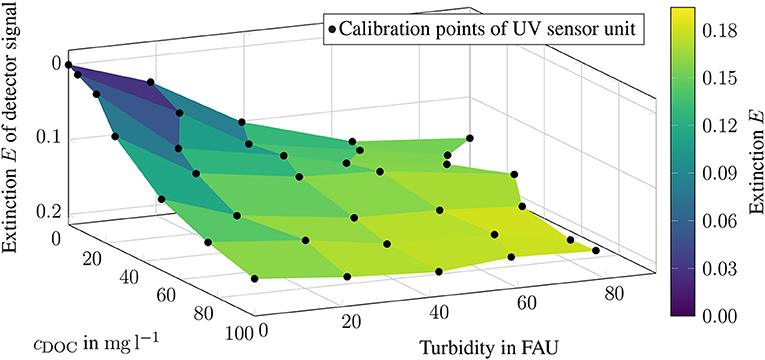
Figure 7. Measured calibration points of the UV sensor represented as extinction values E, plotted on the respective DOC concentration and turbidity. The color yellow represents high detector signals, while dark blue represents low detector signals.
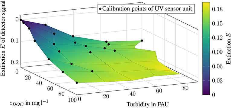
Figure 8. Revised calibration points of the UV sensor unit represented as extinction E, plotted on the respective DOC concentration and corresponding turbidity. The color yellow represents high detector signals, while dark blue represents low detector signals.
3.1.1. Turbidity Compensation
Based on the revised calibration points, a set of calibration curves can be determined. Equation (6) characterizes the linear relationship between the IR sensor signal and various turbidity values and has a measure of determination of R2 = 0.943.
With R2 = 0.948, Equation (7) shows the linear relation between the UV sensor signal and different DOC concentrations.
The calibration curve (see Equation 8) shows the relation between the UV sensor signal and different turbidity values with R2 = 0.932.
However, despite the knowledge of turbidity, it is by far not trivial to deduce the correct content of dissolved organic material in water. For clarification, an approach for turbidity compensation is shown below.
For the different turbidity levels, the relationship between EUV and cDOC is shown in Figure 9.
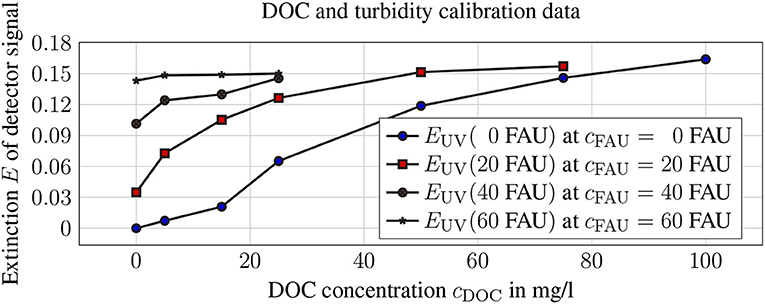
Figure 9. Extinction EUV of the UV detector signal in relation to DOC concentration and the corresponding turbidity values.
The following calibration curves are calculated and converted into cDOC. By inserting the UV detector signal value EUV into the equation with the corresponding turbidity, cDOC can be calculated directly. The differences between compensated and produced DOC values are greatest at cDOC = 15.25 mg l−1.
The compensated measured DOC concentrations correlate closely with more than 90 % regarding the produced DOC concentration of the calibration media. Compared to the uncompensated values, the correlation increased by more than 45 % (see Table 4).
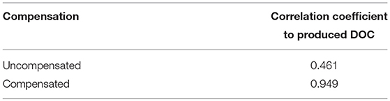
Table 4. Correlation coefficients using compensated and uncompensated values.
3.2. Field Measurements
The advantages of the proposed approach were demonstrated based on a case study. For better readability, the results of the measurement campaigns are presented separately. However, for the sake of completeness, all results and measured values of the monitoring campaigns are listed in the form of tables in the Supplementary Material of this article.
3.2.1. Monitoring Campaign Lake Cospuden, Leipzig
In Figure 10 the raw values of the UV and IR channel in V are plotted as a map. The results of the first campaign carried out on July 2, 2016 are shown in Figures 10A,C. In Figures 10B,D the map view of the monitoring data of the second campaign carried out on July 22, 2016 are given.
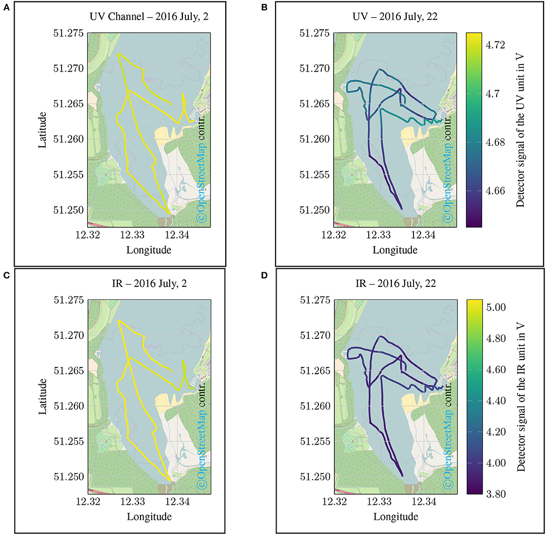
Figure 10. Spatial plot of the UV detector Signal, which corresponds to the DOC content. The data were gathered using a small sailing boat at the Lake Cospuden close to the city of Leipzig (Lake Cospuden, Leipzig, Saxony, Germany). (A) and (C) are showing the results of the campaign carried out on 2 July, 2016. (B) and (D) are containing the results of the campaign carried out on 22 July, 2016. Shown are the pure measurements in V of the optical UV channel (λ = 254 nm). Low values in this representation mean a stronger light attenuation due to increased DOC content.
In addition to proving the field suitability of the developed measuring device, the field tests have also shown that direct feedback in the field, e.g., in the form of a web map display, is of great advantage. Thus, initial statements about distribution patterns can already be made during data collection. Following the idea of Assissted Monitoring, it was possible, for example, to sample areas that appear particularly interesting again or more intensively. Conventional monitoring strategies offer this possibility only to a limited extent.
Even though the data obtained represent the raw measured values of the IR and UV channels, some ecosystem relationships can still be identified as shown in Figure 10. Since no comparative samples were taken during the measurement campaigns for the laboratory analysis of water quality, only quantitative peculiarities will be discussed in the following. This is sufficient for the evaluation of the prototype and the proof of field suitability. With regard to the measurement results of the UV channel, it is noticeable that the values collected during the first measurement campaign (July 2, 2016) were significantly higher than in the second campaign on July 22, 2016 (see Figures 10A,B). With regard to the calibration tests previously carried out in the laboratory, it can therefore be deduced that the extinction as a result of an increased DOC concentration must have been considerably higher at the time of the second measurement campaign.
A similar situation applies to the IR channel. The results for the IR channel also show that there are clear differences in the water status with regard to turbidity (see Figure 10D). As shown in the previous laboratory test, the spectral attenuation in the UV range can also be influenced as a result of increased turbidity. It is not yet possible to determine conclusively from the initial measurements whether the measurement results are due to increased turbidity or an increased DOC concentration. However, supplementary reference measurements at selected points could be used to describe these correlations more precisely in further studies.
3.2.2. Monitoring Campaign Urban Streams, Leipzig
In a second campaign it should be investigated whether the developed measuring system can also be used in very small water systems since small bodies of water such as streams or ditches can only be measured with great effort using conventional methods. However, mobile monitoring approaches for small bodies of water pose an additional challenge. For this purpose, a canoe trip along the Floßgraben, the Pleiße and to the Elster in the urban area of Leipzig was carried out (2016 August, 19). These changed requirements for the monitoring task should show that the measurement system is suitable for a holistic monitoring approach. The results of the measurement campaign are shown in Figure 11.
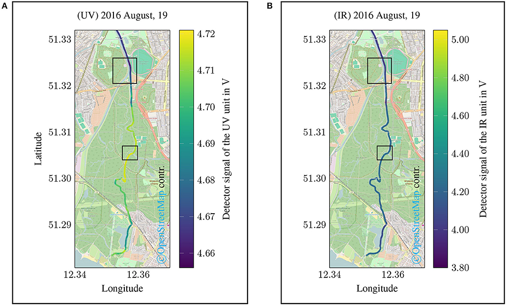
Figure 11. Spatial data plot of a monitoring campaign along a river course (Floßgraben, Pleiße, Elster) in the city area of Leipzig, Saxony, Germany (2016 August, 19). (A) shows the detector signal of the UV channel corresponding to the DOC content. The results of the IR channel are shown in (B). For both representations, lower values indicate a stronger attenuation due to an increased DOC content or increased turbidity.
For the this campaign, the results of the UV channel show a greater dynamic (see Figure 11A) than the values for turbidity (see Figure 11B). Due to the fact that the temperature is also recorded in the measuring system, statements can also be made regarding the thermodynamic properties of the water body. It should be noted that temperature differences in the size of (△ ϑ4 °C) occur particularly during the measuring campaign (see Figure 12).
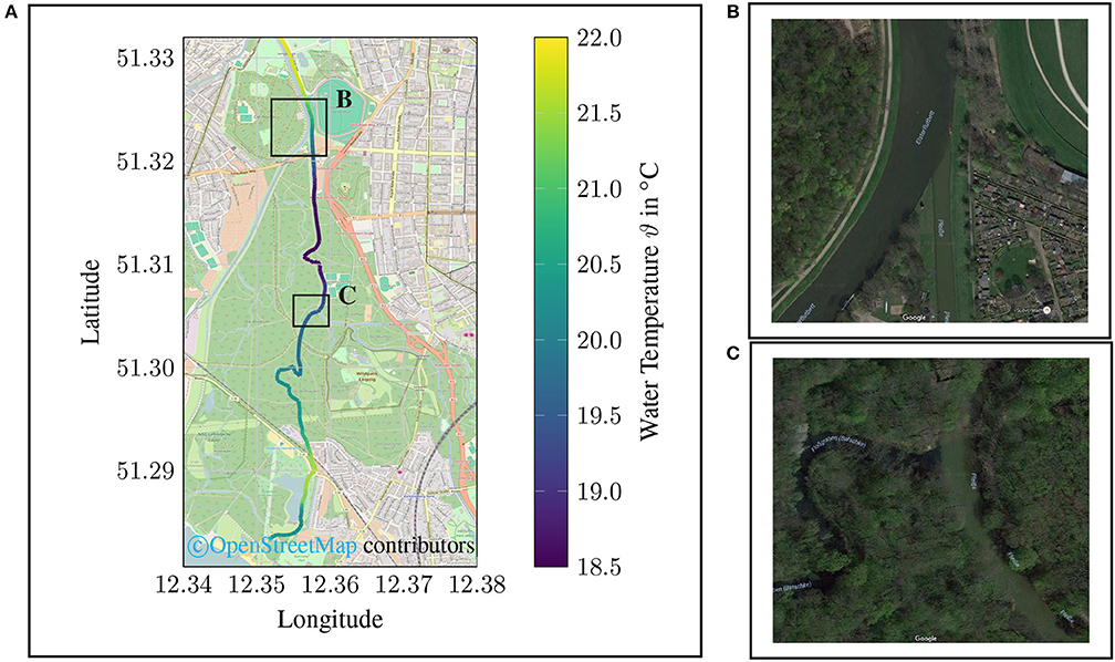
Figure 12. Temperature data of mobile monitoring campaign along a river course (Elstermühlgraben, Pleiße, Elster) in the city area of Leipzig, Saxony, Germany (2016 August, 19). In (A) the spatial plot of the water temperature is given. Two squares are indicating points of special interest. (B) marks the estuary of the Elstermühlgraben into the Pleiße and (C) the estuary of the Pleiße into the Elster. (B retrieved from https://goo.gl/maps/qQyVoWTnV4J2; C retrieved from https://goo.gl/maps/QLphRa7QgGA2).
4. Discussion
The monitoring of DOC content by determining the spectral absorption coefficient at λ = 254 nm is a proven method. Even if there are several established probes on the market, an inexpensive in-situ probe for large area applications is not yet available. The prototype of the in-situ probe presented in this paper shows a general functionality and promising characteristics. The optical UV sensor unit for measuring DOC values and the IR sensor unit for measuring turbidity can be classified as suitable for photometric measurements. The hardware required for setting up the sensors is manageable thanks to the LEDs used. The costs are also lower compared to previously installed mercury vapor lamps. At the same time, energy efficiency has been increased and applicability improved by reducing the size.
There are some limitations with regard to the laboratory analytical evaluation and calibration of the sensor system. Since the relative standard deviation of the compensated values is higher than 100 %, it is not yet possible to measure precisely compensated DOC concentrations. However, since the correlation between the compensated measured DOC values and the real DOC values is significantly higher than the correlation between the uncompensated and the real DOC values, the turbidity compensation method has led to an improvement of the sensor readings. Possible causes for the high standard deviations lie in the calibration method or the electronic components of the probe used. In addition, formazine could be used as a turbid material because talcum powder solutions were difficult to homogenize. The accuracy of the compensated DOC values can be improved by adding additional turbidity values to the calibration. The range in which DOC concentration and absorbance are linear is very small for this prototype. A light source with a higher radiant power allows measurements of higher DOC concentration and turbidity values. Thus, at higher concentrations, the measurement signal reaches the saturated range and the linear range of the calibrated range becomes larger. By using a “UVLUX250-5” LED, the radiation power can be increased from 0.3 mW to more than 3 mW compared to the currently installed LED. Reducing the distance between the emitter and detector can also increase the maximum measurable concentrations. A further limitation can be found in the lack of verification by means of accompanying measurements during the mobile monitoring campaigns. This was not included in the basic feasibility study presented in this paper. For later studies, however, reference measurements should be made using established laboratory analytical methods and appropriate sampling, and the results and sensor performance should be evaluated accordingly.
The differences shown between the individual days (cf. Figures 10A,B) cannot be clearly justified in the context of the present study, as comparative measurements are also lacking here. Nevertheless, the prove was made that the presented measurement system is able to show spatial differences with little methodical effort and in near real time. Compared to conventional sampling and subsequent laboratory analysis, there is a considerable advantage in terms of time, method and therefore also in financial terms.
What has not yet been satisfactorily solved in the context of this study is the integration of sufficient temperature compensation to eliminate signal deviations due to temperature changes. Both the semiconductor elements used (emitter and detector) and the remaining electronics show temperature dependencies. This should be taken into account in subsequent studies.
In summary, the work shows that a measurement of DOC with a dual wavelength method at λ = 254 nm and λ = 860 nm can be realized by using LEDs, photodiodes and several low cost components. Additional experiments are necessary to improve the accuracy of the measurement. The use of more suitable components and an improvement of the calibration method are possible next steps. However, the open-source-based approach also offers the possibility of extending the range of functions and making additional optimization.
5. Conclusion
In addition to sensor and system development, the introduction of a holistic sampling theorem (OSE) is an essential part of this work (Schima et al., 2017). Through the combination of the monitoring paradigm and the consistent sensor development from the beginning, an unprecedented measurement system was achieved with regard to its functionality. Integrated functions for controlling the emitter intensity by changing the forward current or the pulse width modulation as well as the adjustable detector sensitivity by changing the integration time enable sophisticated functions such as autocalibration routines or adaptive system behavior. Therefore, this paper describes the structure of a modular and adaptive optical sensor concept, which opens the possibility of a fast and service-oriented environmental monitoring.
However, in order to show the feasibility of the sensor system, different initial field measurements campaigns were carried out in the area of the city of Leipzig, Saxony, Germany. A major advantage of the system is seen in its small size and low weight. This allows to carry out appropriate measurements even with small boats such as canoes or small sailing boats. Especially for shallow waters, where such measurements are often missing, this is an important addition to conventional monitoring strategies. In addition, a comparative study has shown that the sensor system presented delivers results that correspond to the laboratory analytical standard method with a laboratory photometer. Thus, the measurement quality for the proposed application is considered acceptable.
The results confirm that the prototype of the sensor system represents a promising approach that meets the requirements and specifications outlined in the introduction to this work. Therefore, the sensor system provides a fast and useful method to support and improve future environmental monitoring applications, especially for the investigation of areas not yet accessible with conventional monitoring technologies.
Data Availability
The raw data supporting the conclusions of this manuscript will be made available by the authors, without undue reservation, to any qualified researcher.
Author Contributions
RS, MP, PD, and TG contributed conception and design of the study. RS was responsible for the design of the sensor system and the development of the electronics. The laboratory study was conceptually developed by RS. The laboratory work was carried out by SK. The results of the laboratory tests were evaluated by SK and RS. TG organized the database, the web service and the visualization. RS carried out the field tests and performed the statistical analysis. RS and TG wrote the first draft of the manuscript. All authors contributed to manuscript revision, read, and approved the submitted version.
Conflict of Interest Statement
The authors declare that the research was conducted in the absence of any commercial or financial relationships that could be construed as a potential conflict of interest.
Acknowledgments
We acknowledge financial support by Deutsche Forschungsgemeinschaft and Universität Rostock within the funding programme Open Access Publishing.
Supplementary Material
The Supplementary Material for this article can be found online at: https://www.frontiersin.org/articles/10.3389/feart.2019.00184/full#supplementary-material
References
Bass, M., Van Stryland, E., Williams, D. R., and Wolfe, W. L. (eds.). (1995). Handbook of Optics, Volume I: Fundamentals, Techniques, and Design, 2 Edn, Vol. 1. New York, NY: McGraw-Hill, Inc.
Brewin, R. J. W., Hyder, K., Andersson, A. J., Billson, O., Bresnahan, P. J., Brewin, T. G., et al. (2017). Expanding aquatic observations through recreation. Front. Mar. Sci. 4:351. doi: 10.3389/fmars.2017.00351
Chapman, D. (ed.). (1996). Water Quality Assessments - A Guide to Use of Biota, Sediments and Water in Environmental Monitoring, 2 Edn. London: E & FN Spon.
Clifford, N. J., Richards, K. S., Brown, R. A., and Lane, S. N. (1995). Laboratory and field assessment of an infrared turbidity probe and its response to particle size and variation in suspended sediment concentration. Hydrol. Sci. J. 40, 771–791. doi: 10.1080/02626669509491464
[Dataset] DIN 38404-3 (2005). Deutsche Einheitsverfahren zur Wasser-, Abwasser- und Schlammuntersuchung - Physikalische und Physikalisch-Chemische Kenngrößen (Gruppe C) - Teil 3: Bestimmung der Absorption im Bereich der UV-Strahlung, Spektraler Absorptionskoeffizient (C 3).
[Dataset] DIN EN 1484 (1997). Wasseranalytik - Anleitungen zur Bestimmung des Gesamten Organischen Kohlenstoffs (TOC) und des Gelösten Organischen Kohlenstoffs (DOC).
Guo, L., Santschi, P. H., and Warnken, K. W. (1995). Dynamics of dissolved organic carbon (DOC) in oceanic environments. Limnol. Oceanogr. 40, 1392–1403. doi: 10.4319/lo.1995.40.8.1392
Hoge, F. E., Vodacek, A., Swift, R. N., Yungel, J. K., and Blough, N. V. (1995). Inherent optical properties of the ocean: retrieval of the absorption coefficient of chromophoric dissolved organic matter from airborne laser spectral fluorescence measurements. Appl. Opt. 34, 7032–7038.
Huang, J., Liu, H., Tan, A., Xu, J., and Zhao, X. (1992). A dual-wavelength light-emitting diode based detector for flow-injection analysis process analysers. Talanta 39, 589–592. doi: 10.1016/0039-9140(92)80065-L
Hut, R., Tyler, S., and van Emmerik, T. (2016). Proof of concept: temperature-sensing waders for environmental sciences. Geosci. Instrum. Methods Data Syst. 5, 45–51. doi: 10.5194/gi-5-45-2016
Kolka, R., Weishampel, P., and Fröberg, M. (2008). “Measurement and importance of dissolved organic carbon,” in Field Measurements for Forest Carbon Monitoring, ed C. M. Hoover (Dordrecht: Springer), 171–176.
Liu, H., and Dasgupta, P. K. (1994). Dual-wavelength photometry with light emitting diodes. Compensation of refractive index and turbidity effects in flow-injection analysis. Anal. Chim. Acta 289, 347–353. doi: 10.1016/0003-2670(94)90011-X
Lockridge, G., Dzwonkowski, B., Nelson, R., and Powers, S. (2016). Development of a low-cost arduino-based sonde for coastal applications. Sensors 16:528. doi: 10.3390/s16040528
Moore, C., Barnard, A., Fietzek, P., Lewis, M. R., Sosik, H. M., White, S., et al. (2009). Optical tools for ocean monitoring and research. Ocean Sci. 5, 661–684. doi: 10.5194/os-5-661-2009
Preisendorfer, R. W. (1976). Hydrologic Optics. Volume 1. Introduction. Technical Report, Honolulu, HI: U.S. Dept. of Commerce, National Oceanic and Atmospheric Administration, Environmental Research Laboratories, Pacific Marine Environmental Laboratory.
Schima, R. (2018). A fast method for mobile in-situ monitoring of optical properties in aquatic environments (Unpublished thesis). University of Rostock, Rostock, Germany.
Schima, R., Goblirsch, T., Salbach, C., Franczyk, B., Aleithe, M., Bumberger, J., et al. (2017). “Research in progress: implementation of an integrated data model for an improved monitoring of environmental processes,” in Business Information Systems Workshops. Lecture Notes in Business Information Processing (Cham: Springer), 332–339. doi: 10.1007/978-3-319-52464-1_30
Seibert, J., Strobl, B., Etter, S., Hummer, P., and van Meerveld, H. J. I. (2019). Virtual staff gauges for crowd-based stream level observations. Front. Earth Sci. 7:70. doi: 10.3389/feart.2019.00070
Skrabal, P. (2009). Spektroskopie: Eine Methodenübergreifende Darstellung vom UV- bis zum NMR-Bereich (Zürich: vdf Hochschulverlag AG).
Keywords: photonic sensing, in-situ measurements, assisted monitoring, attenuation sensor, internet of things, water quality
Citation: Schima R, Krüger S, Bumberger J, Paschen M, Dietrich P and Goblirsch T (2019) Mobile Monitoring—Open-Source Based Optical Sensor System for Service-Oriented Turbidity and Dissolved Organic Matter Monitoring. Front. Earth Sci. 7:184. doi: 10.3389/feart.2019.00184
Received: 28 February 2019; Accepted: 01 July 2019;
Published: 17 July 2019.
Edited by:
Peter M. Marchetto, University of Minnesota Twin Cities, United StatesReviewed by:
Tim van Emmerik, Delft University of Technology, NetherlandsAhmed M. ElKenawy, Mansoura University, Egypt
Copyright © 2019 Schima, Krüger, Bumberger, Paschen, Dietrich and Goblirsch. This is an open-access article distributed under the terms of the Creative Commons Attribution License (CC BY). The use, distribution or reproduction in other forums is permitted, provided the original author(s) and the copyright owner(s) are credited and that the original publication in this journal is cited, in accordance with accepted academic practice. No use, distribution or reproduction is permitted which does not comply with these terms.
*Correspondence: Robert Schima, robert.schima@uni-rostock.de