
Abstract
In clinical ion beam therapy, protons as well as heavier ions such as carbon are used for treatment. For protons, β+-emitters are only induced by fragmentation reactions in the target (target fragmentation), whereas for heavy ions, they are additionally induced by fragmentations of the projectile (further referred to as autoactivation). An approach utilizing these processes for treatment verfication, by comparing measured Positron Emission Tomography (PET) data to predictions from Monte Carlo simulations, has already been clinically implemented. For an accurate simulation, it is important to consider the biological washout of β+-emitters due to vital functions. To date, mathematical expressions for washout have mainly been determined by using radioactive beams of 10C- and 11C-ions, both β+-emitters, to enhance the counting statistics in the irradiated area. Still, the question of how the choice of projectile (autoactivating or non-autoactivating) influences the washout coefficients, has not been addressed.
In this context, an experiment was carried out at the Heidelberg Ion Beam Therapy Center with the purpose of directly comparing irradiation-induced biological washout coefficients in mice for protons and 12C-ions. To this aim, mice were irradiated in the brain region with protons and 12C-ions and measured after irradiation with a PET/CT scanner (Siemens Biograph mCT). After an appropriate waiting time, the mice were sacrificed, then irradiated and measured again under similar conditions. The resulting data were processed and fitted numerically to deduce the main washout parameters.
Despite the very low PET counting statistics, a consistent difference could be identified between 12C-ion and proton irradiated mice, with the 12C data being described best by a two component fit with a combined medium and slow washout fraction of 0.50 ± 0.05 and the proton mice data being described best by a one component fit with only one (slow) washout fraction of 0.73 ± 0.06.
Export citation and abstract BibTeX RIS
1. Introduction
The in-vivo verification of the beam range and applied dose is increasingly considered an important aspect for the improvement of treatment possibilities in ion beam therapy. For this purpose, positron emission tomography (PET) treatment verification has already been clinically investigated at different centers (Hishikawa et al 2002, Enghardt et al 2004, Parodi et al 2007b, Nishio et al 2010, Zhu et al 2011, Bauer et al 2013). Using a PET scanner, the irradiation-induced activity in the patient is measured. For protons, the activity is only induced by fragmentation reactions in the target (target fragmentation), while for heavy ions (Z ⩾ 5), activation is additionally induced by fragmentation of the projectile (further referred to as autoactivation). The measured PET data must be compared with an expected PET distribution, which can be calculated using Monte-Carlo (MC) simulations with the assumption of a correct treatment application, to validate the planned particle range in tissue (Poenisch et al 2004, Parodi et al 2007a, Zhu et al 2011, Bauer et al 2013). For PET-measurements, three main workflows exist (Shakirin et al 2011): an approach with the detector implemented at the treatment site (online) and two approaches with the PET-scanner spatially separated from the treatment site, either within (in-room) or outside (offline) the treatment room. Especially for the offline workflow, which causes a certain time delay between activity induction and measurement, biological washout effects become important in calculating the correct expectation. To this aim, the washout can be expressed mathematically in terms of biological decay coefficients, also called washout coefficients, which can be used in modeling to identify the fraction of physically produced β+-emitters disappearing at an accelerated rate due to the combined effect of physical decay and biological clearance (Parodi et al 2007b, Parodi et al 2008).
Pioneering experiments carried out by Mizuno et al with radioactive 10C- and 11C-ion beams implanted in rabbit brain and muscle have motivated a description consisting of three biological decay components (Mizuno et al 2003). More recent experiments with 11C and 12C beams in rat and human brain, respectively, also confirmed medium and slow washout component, consistent with the earlier findings with radio-active beams in rabbits (Helmbrecht et al 2013, Hirano et al 2013). However, until now, no study has reported a direct comparison of washout coefficients for irradiation with proton and stable carbon ion beams, although the question of whether a difference can be seen is clinically relevant. Although biological parameters deduced from animal data are not necessarily representative of human metabolism and internal biology and cannot be directly translated in medical practice, they allow probing of this question directly via irradiation and PET acquisition of the same subject under living and dead conditions. Here, we present our experimental work with the objective of shedding insights on the dependency of the washout coefficients on the primary projectile for clinically used radiation qualities, specifically questioning the typical assumption of ion-independent washout parameters.
2. Materials and methods
2.1. Experimental procedure
The experiment was carried out at the Heidelberg Ion Beam Therapy Center (HIT). Ten 6–8 week-old female VM/DK mice (DKFZ animal core facility) were selected. Animal work was performed according to rules outlined by the local and governmental animal care committee instituted by the German government (Regierungspraesidium, Karlsruhe). For the first part of the experiment, the mice were anaesthetized, fixed in pairs and aligned at the isocenter of the irradiation site using a laser system. The irradiation target was the brain, where tumors (spontaneous murine astrocytoma (SMA)-560 cells) had developed in the right hemisphere. SMA-560 is characterized by the formation of tumor bulk with massive angiogenesis (perfusion), necrotic regions, invasive borders and a stroma-rich microenvironment. After irradiation, the mice were transported to a PET/CT scanner (Siemens Biograph mCT with UltraHD option) located approximately 100 m from the experimental treatment room. There, the induced activity as well as anatomic information about the mice was acquired via PET and CT measurements, respectively (figure 1). After a waiting time of at least two hours, so that residual activity could be considered negligible, the mice were sacrificed, irradiated and measured again under similar conditions. In total, the procedure was carried out for five pairs of mice.
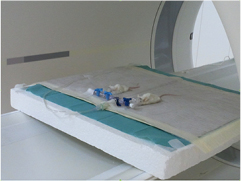
Figure 1. Pairwise alignment of two sedated mice after irradiation during the PET measurement at the PET/CT scanner.
Download figure:
Standard image High-resolution imageThe beams were generated using the linac-synchrotron combination at the HIT facility. Comparable treatment plans were designed with protons and 12C-ion beams, in order to irradiate the brain with a homogeneous dose distribution from a spread-out Bragg peak (SOBP) target volume of 10 mm lateral and 5 mm longitudinal extension in water, delivering 30 Gy physical dose (figure 2). Using the active raster scan system, the two SOBPs were delivered at once to each mice pair, immobilized in a custom-designed plexiglas holder, with special care to adjust the lateral position of the treatment field to the middle of the mice skull and the beginning of the SOBP at the mice entrance skin surface using a 10 cm thick plexiglas degrader along the horizontal beam direction. Due to the synchrotron-based beam delivery, the irradiation consisted of a few particle spills of different energy. Specifically, four iso-energy slices (E = 241.8 − 246.6 MeV u−1) with an average lateral beam size of 4.4 mm (FWHM) were delivered with carbon ions for each SOBP, whereas six energy slices (E = 125.7 − 128.7 MeV u−1) with an average spot size of 12.8 mm (FWHM) were used for protons. Reproducibility of the lateral position of the irradiation field was in the order of ± 1 mm, which is somewhat worse than the achievable accuracy of ± 0.5 mm in the positioning of individual mice with the help of a holder and room laser. Relevant parameters for evaluation are total irradiation time (Tirr), elapsed time between the end of irradiation and beginning of PET-measurement (Toff) and the length of PET-measurement (TPET) (table 1). The times between the end of irradiation and the beginning of PET-measurement were recorded using a stop watch and duration of PET-measurement was defined beforehand in the examination protocol, where intervals of 30 min were typically chosen, with 60 min and 90 min for some mice to test the influence of a longer reconstruction time.
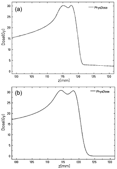
Figure 2. Planned spread-out Bragg peak (SOBP) target volume of 10 mm lateral and 5 mm longitudinal extension in water for (a) 12C and (b) proton irradiation.
Download figure:
Standard image High-resolution imageTable 1. Irradiation time, Tirr, time between end of irradiation and beginning of PET, Toff and PET acquisition time, TPET. The mice pairs are labeled by number according to the order of measurement and by de for dead and al for alive.
| Mouse (12C) | 1de | 1al | 2de | 2al | 3de | 3al |
|---|---|---|---|---|---|---|
| Tirr [s] | 36 | 33 | 35 | 32 | 39.6 | 40.9 |
| Toff [s] | 263 | 362 | 185 | 316 | 181.3 | 192.7 |
| TPET [min] | 30 | 30 | 30 | 30 | 60 | 90 |
| Mouse (protons) | 4de | 4al | 5de | 5al |
| Tirr [s] | 86 | 102 | 84.5 | 91 | ||
| Toff [s] | 212 | 255 | 158.6 | 203 | ||
| TPET [min] | 60 | 90 | 90 | 90 |
For diagnostic PET-investigations, the decay constant of the injected radionuclides is well-known. Hence, there is a radionuclide-specific correction implemented in the scanner. To prevent this correction for the unknown mixture of isotopes, 22Na, with a half life of 2.6 y, was chosen as the applied isotope (Bauer et al 2013).
2.2. Data handling
CT images (also used for attenuation and scatter correction of the PET data) were reconstructed with a pixel size of circa 0.605 mm and a slice thickness of 0.6 mm. The raw PET list mode data were reconstructed in two different ways: Static PET images were derived from averaging the activity values over the total measurement time. For dynamic PET images, the PET data sets were subdivided into shorter time frames over which the activity data were averaged. After testing a variety of configurations and algorithms, the time intervals (3 × 60 s, 4 × 180 s, 3 × 300 s) were chosen. All PET data were reconstructed using the filtered back projection (FBP) algorithm because of enhanced activity consistency between static and dynamic PET images (see section 2.3.1), with a pixel size of circa 1.06 mm and the same CT slice thickness of 0.6 mm. The resulting image data were saved in the digital imaging and communications in medicine (DICOM) format. Volumes of interest (VOI) containing the tumour and a large fraction of the brain were drawn by hand on the basis of the CT data using the scanner software syngo for quantitative evaluation. In this process, special care was taken to exclude regions close to the bone, resulting in VOI volumes of approximately 80 mm3 (figure 3).
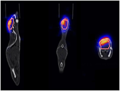
Figure 3. Overlapped PET, VOI and CT data for an exemplary mouse.
Download figure:
Standard image High-resolution imageTo handle the image files, networks created in the software environment MeVisLab (MeVis Medical Solutions AG) were used, whose basic scaffold was developed at HIT (Unholtz et al 2011). The networks provided the possibility of overlapping and evaluating PET and CT images as well as the VOIs (figure 3). Using this software, the activity values of each voxel within the VOI were extracted from the PET images, summed and averaged. Hence, every time frame was assigned one value of activity, which was not dependent on location within the VOI, but only on the average activity of the VOI within the selected time frame. All evaluations of numerical data as described in section 2.3 were implemented using Matlab software (The MathWorks, Inc.). Additionally, the elemental composition of the tissue within the VOI was quantified by converting the Hounsfield units (HUs) of the DICOM CTs using a stoichiometric calibration table (Schneider et al 2000).
2.3. Data analysis
According to the method proposed by Mizuno and co-workers (Mizuno et al 2003), the experiment was evaluated by first estimating the activity induced purely by irradiation from the data of the dead mice (further referenced as physical activity) and subsequently evaluating the biological washout from the data on the living mice. In both cases, the desired quantities were obtained by fitting the averaged activities in the VOI of the dynamic PET as a function of time using a weighted least squares fit with the assumption of an activity signal governed by Poisson statistics.
Different fit scenarios were evaluated, which are discussed in the following.
2.3.1. Physical activity in the dead mice.
The physical activity Aphys of radionuclides as a function of time is described by the formula

where λi is the half life of the isotope i, x = t − t*, t is the time, t* is the time at the beginning of data acquisition (with respect to time 0 at the end of irradiation) and Ai is the fitting parameter, estimating the activity of the isotope i. Using the data of the dead mice, Ai was determined. Ai(t*) can be expressed in normalized form as
To obtain a valid estimation for the physical activity, the dominant isotopes i as well as appropriate time intervals for the dynamic PET reconstruction had to be chosen correctly. The isotopes chosen for Aphys were 11C and 15O in all cases, as additional isotopes could not be detected properly by the fit, most likely due to their negligible contribution. In fact, implementations attempting to account for additional isotopes such as 13N or 38K gave physical inconsistencies as, for example, negative Ai values. Hence, referring to formula (2), P(t*) denotes the relative share of 11C isotopes at the start of the scan while the share of 15O is deduced as 1 − P(t*).
For the choice of time intervals, a compromise had to be found between increasing the information density for the time evaluation of the data and decreasing the error due to low counting statistics in short time intervals. For verification of the chosen settings, the mean activity < A > was calculated as

with TPET being the whole interval of measurement and Ai(t*) the results from the dynamic data analysis. The result for < A > was then compared with the value obtained from the static PET.
2.3.2. Mathematical representation of the biological washout.
The model used by Mizuno and co-workers estimates the washout in terms of so called biological half times. The model to describe the effective decay for the living mice Aeff can be written as

with

where Mf, Mm and Ms are the fractions of the respective fast, medium and slow components and correspond to fast  , medium
  and slow
  decay constants, which are speculated to be due to fast blood flow, microcirculation and trapping of the isotope by the stable molecules of the organs, respectively (Mizuno et al 2003). For a functioning model, the fractions must satisfy the constraint

Thus, if there is no biological decay, all biological decay constants are zero (i.e. the corresponding half times are infinite) and Aeff does not differ from Aphys. As the fast component was estimated to be a few seconds by Mizuno et al, while Toff varied between 2.5 min and 4.5 min in the HIT experiments (table 1), the expression Mf·exp(−λft) was set to zero and hence neglected in equation (5), giving a two component function.
2.3.3. Physical activity in the living mice.
As can be seen in table 1, there are fluctuations in the irradiation times; in particular, the transfer times Toff differ for dead and live mice. The effect on the live mice is due to a more time-consuming procedure required when handling live animals. As it was desired to transfer the result for Aphys from the dead to the living mice, effects due to the different time courses of irradiation and imaging must be compensated. This can be achieved by using the concept of a production rate Ri of isotopes i during irradiation. Unfortunately, it was not possible to recalculate exactly the real applied field, due to missing logged information and varying beam energy over the few delivered spills. Hence, approximations were used. To estimate the uncertainties associated with these approximations, the production rate was calculated twice. The first calculation used the approximation of continuous irradiation with constant beam parameters (Parodi et al 2002)

with Tirr being the time at the end of irradiation. A more refined approximation took into account the pulsed structure of the synchrotron irradiation by estimating a repetition of an equal number of spills and pauses with fixed tspill and tpause:

where tspill is the average length of the spill and tpause is the average time between. Although this mathematical formalism neglects in both cases that the spills may have different energies, the model can be regarded as a reasonable approximation since the number of spills is small (five to 15) and the extension in depth of the treatment field is very limited. Ai(Tirr) can be calculated easily from the fit of the dead mice data using the decay law, thus yielding the production rate Ri for the dead mice data. This allows estimation of the physical activity in the living mice by rearranging equations (7) or (8), respectively, to solve for Ai, plugging in Tirr of the living mice (table 1) and the isotope production rates Ri deduced from the dead mice data. As the same approximation was performed in two steps, calculating backwards from the production rate (for the dead mice) and then projecting this forwards to the live mice, the effect of the different energy spills is additionally reduced. Hereby, the unknown biological decay during the relatively short irradiation is neglected. For verification of this approximation, the values for biological decay, once determined with the proposed analysis, can be inserted in the following formula to evaluate their impact with respect to the calculation that neglects the biological decay during the short irradiation time:

with λb being the biological washout coefficient determined from the fit and and Mb the corresponding fraction for the accessible medium and slow components. This is a reasonable approximation, as a fast washout component of only a few seconds as reported by Mizuno et al would give an already negligible contribution for the shortest irradiation time of circa 30 s (see table 1). The values for Aphys · (Mm + Ms) and Aphys,corrected, derived from equations (7)–(9) were finally compared at the end of irradiation Tirr.
2.3.4. Fit approaches.
Several types of function showed to be relevant for evaluation. Most important, a two component fit function Afit(x) of the form

where x = t − t* and the fitting parameters a1 = Ms, a2 = Mm, b1 = Ts and b2 = Tm with the biological half times Ts and Tm.  is the normalized (see equation (2)) representation of Aphys (equation (1)),

The total physical activity (i.e. the activity that would exist without any biological decay) at the beginning of measurement (Aphys(t = t*)) is referred to as A*, which was deduced by adjusting the data of the dead mice to the living mice as described in section 2.3.3.
For reasons of fit stability, in some fits a two component function was used, where the slow decay constant was approximated to be zero (i.e. half life time going to infinity), giving

with a1 = Ms, a2 = Mm, and b1 = Tm.
A one component function of the form

with a1 = Ms and b1 = Ts, was also implemented for cases where no medium component was evident. When necessary, constraints were set in the form of upper and lower boundaries for the fitting parameters to guarantee physically plausible results.
A third approach, overcoming the uncertainties of the  evaluation at the expense of decreasing fit stability, is to approximate the function Aeff with an additional free fit parameter under the assumption of the two dominant isotopes 11C and 15O

The fit-function can be written in the form
resulting in five fit parameters a1 = MsA011C,  , a3 = Ts,
  , a5 = Tm, with A0 corresponding to the activity at the beginning of the PET measurement t*. To enhance the probability of getting physically plausible results, upper and lower boundaries for the parameters were set. As the additional free parameter is leading to a higher fit instability, this fit was only used for verification.
Additionally, the approach of fitting the slow component first and afterwards the medium component, as implemented by Mizuno and colleagues, was tested. For this successive approach the data was first fitted at late times, to estimate solely the slow decay component with a stable one component fit. In a second step, the slow decay constant was fixed to the estimated value and the whole data set was fitted again using a one component fit.
Finally, a collective fit was used in order to attempt determining global coefficients that would give a reasonable fit for multiple mice, instead of optimizing data for individuals. For this purpose, the two component fit (equation (10)) was used. A collection of N mice-datasets was chosen (see section 3.2). For each step of the fit-iteration, a curve with identical parameters a1, a2, b1, b2 was plotted for every dataset and only Aphys was adapted for each curve according to the individual mice measurements. The weighted squared distances of the N curves to the data points of the N datasets were summed up and this collective sum was then minimized by the weighted least squares iteration. To ensure equal influence of every dataset, all individual squared distances were divided by their minimum squared distance from the individual fits, before being summed up.
2.3.5. Comparison to static PET for alive mice.
For verification, the average activity deduced from the fit results of the dynamic acquisitions were compared to the static PET of the living mice, using the formula

where the index p denotes the physical and b the biological parameters, while Airr,p refers to the estimated activity at the end of irradiation.
2.3.6. Sensitivity study on the P-values.
To test the validity of transferring Aphys (and hence  ) from the dead to the living mice, the stability of the resulting fitting coefficients was evaluated by changing the normalized value of 11C activity at the beginning of measurement, P(t*), by ± 10% and fitting the data sets again.
2.3.7. Estimation of standard errors of the fit parameters.
The error of each fit parameter σp was estimated by the diagonal elements of the covariance matrix Cpp, weighted with the reduced χ2 of the fit, assuming Poisson distribution of the measured data. This gave the expression

where

The degrees of freedom (dof) were obtained by subtracting the number of fit parameters from the number of data points.
3. Results
3.1. Dynamic PET image reconstructions
The dynamic PET reconstruction gave a good consistency with the static PET activity values for the dead mice (table 2). Only the first 30 min of PET data were used for all mice, because no improvement could be seen in the results when taking longer decay intervals.
Table 2. Mean activity determined from the static PET and from the dynamic PET via equation (3) for the dead mice, labelled additionally according to position in the CT (l: left; r: right). The relative deviation ΔS (in %) is given in the last row.
| Mouse (12C) | 1de,l | 1de,r | 2de,l | 2de,r | 3de,l | 3de,r |
|---|---|---|---|---|---|---|
![$< A {{>}_{\text{stat}}}\left[\frac{Bq}{ml}\right]$](https://content.cld.iop.org/journals/0031-9155/59/23/7229/revision1/pmb503541ieqn009.gif) |
703.5 | 654.6 | 618.1 | 672.2 | 418.0 | 344.9 |
![$< A {{>}_{\text{dyn}}}\left[\frac{Bq}{ml}\right]$](https://content.cld.iop.org/journals/0031-9155/59/23/7229/revision1/pmb503541ieqn010.gif) |
699.7 | 650.0 | 619.7 | 675.1 | 416.4 | 339.4 |
| ΔS | 0.5% | 0.7% | 0.3% | 0.4% | 0.4% | 1.6% |
| Mouse (protons) | 4de,l | 4de,r | 5de,l | 5de,r |
![$< A {{>}_{\text{stat}}}\left[\frac{Bq}{ml}\right]$](https://content.cld.iop.org/journals/0031-9155/59/23/7229/revision1/pmb503541ieqn011.gif) |
153.2 | 148.0 | 223.2 | 218.3 | ||
![$< A {{>}_{\text{dyn}}}\left[\frac{Bq}{ml}\right]$](https://content.cld.iop.org/journals/0031-9155/59/23/7229/revision1/pmb503541ieqn012.gif) |
152.0 | 146.6 | 216.5 | 215.5 | ||
| ΔS | 0.7% | 0.9% | 3.0% | 1.3% |
3.2. Selection of mice data
In the data analysis mouse 1l and mouse 3r were excluded due to missing stability of the fit results under change of P(t*) (section 2.3.6). Mouse 4r was excluded due to bad consistency with the static PET for the living mice. For mouse 2l, the most consistent fit was the multiplication of Aphys with a constant. Inspection of the datapoints did not indicate a clear activity decay and inspection of the overlapped PET, VOI and CT showed that irradiation had taken place mostly outside the VOI. Hence, mouse 2l was excluded due to lack of information correlated with the irradiation-induced activity. Therefore, a total of six mice were considered in the final evaluation. The collective fitting was done separately for the 12C and proton irradiated mice data, with 3 datasets for each.
3.3. Washout coefficients
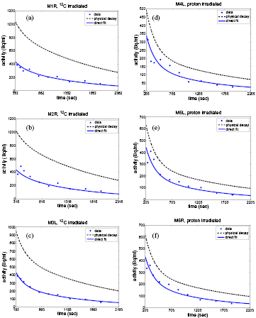
The results for the washout parameters are reported in table 3. The model of continuous irradiation is used for the reported results. All of the selected 12C mice data sets were best fitted by an unconstrained two component fit. Fits that converged to very high Ts are marked by >100 000 and >18 000 in one case. The data sets of mice irradiated with protons were best fitted by an unconstrained one component fit. They gave physically inconsistent values when fitted with an unconstrained two component fit (negative Ms/Mm), while the constrained two component fit converged to the listed one component fit. The successive fit proved to be inconclusive due to the decrease in statistics when starting the fit at least 500 s after irradiation, as required to suppress the medium component. The result of the collective fit gave instead satisfactory results (figure 4) and its comparison to the average and one standard deviation from the separate fits of the individual mice data sets can be seen in table 4.
Figure 4. Results of the collective fit plotted against time with respect to the end of irradiation with 12C-ions (a, b, c) and protons (d, e, f) (see table 1). The physical decay calculated according to section 2.3.3 is shown as a dashed line for comparison. As the method of the collective fit is used, the curves do not give the optimum fit for the individual data points. Still the general time course is well reproduced.
Download figure:
Standard image High-resolution image
Table 3. Results for the washout coefficients: the data of the 12C irradiated mice were fitted by a two component unconstrained fit, the data of the proton irradiated mice by a one component unconstrained fit. The relative deviation between static and dynamic PET ΔS for the alive mice is also reported.
| Mouse | Ts [s] | Tm [s] | Ms | Mm | Ms + Mm | ΔS |
|---|---|---|---|---|---|---|
| 12C | ||||||
| 1r | >18 000 | 322 ± 98 | 0.35 ± 0.01 | 0.10 ± 0.01 | 0.45 | 1.5% |
| 2r | >100 000 | 453 ± 76 | 0.32 ± 0.01 | 0.22 ± 0.01 | 0.55 | 0.5% |
| 3l | >100 000 | 1390 ± 96 | 0.11 ± 0.02 | 0.38 ± 0.02 | 0.49 | 0.1% |
| Protons | ||||||
| 4l | 2775 ± 191 | 0.67 ± 0.01 | 0.67 | 6.4% | ||
| 5l | 2433 ± 168 | 0.76 ± 0.01 | 0.76 | 2.3% | ||
| 5r | 1938 ± 85 | 0.77 ± 0.01 | 0.77 | 2.7% |
Table 4. Results for the collective fits and their comparison to average and standard deviation from the separate fits of the individual mice data sets.
| Ts [s] | Tm [s] | Ms | Mm | Ms + Mm | |
|---|---|---|---|---|---|
| 12C | 3527 | 249.0 | 0.35 | 0.19 | 0.53 |
| From individuals | >100 000 | 722 ± 583 | 0.26 ± 0.13 | 0.23 ± 0.14 | 0.50 ± 0.05 |
| Protons | 2094 | 0.75 | 0.00 | 0.75 | |
| From individuals | 2382 ± 421 | 0.73 ± 0.06 | 0.00 | 0.73 ± 0.06 |
3.4. HU analysis
Using the results of the elemental analysis of the CT images (see tables A1 and A2 in appendix
3.5. Estimation of uncertainties
The comparison of the dynamic with the static PET gave very good consistency for almost all living mice, except mouse 4l,a. Here, the deviation was higher with 6.4% (table 3), likely due to low counting statistics (see figure 4d).
The effects resulting from neglecting the biological decay during irradiation, estimated via equation (9), mostly affected the data sets of mouse 1r and mouse 2r by a raise of Mm + Ms of 3.4% and 2.4%, respectively. The other mice were affected by changes smaller than 1.5% . In all cases, the estimation of P(t*) did not change significantly due to biological washout during irradiation (<0.1%). Comparing the examined approximations for irradiation, the model of continuous irradiation (equation (7)) and the model of pulsed delivery of equal spills and pauses (equation (8)) gave nearly identical results under the condition that the sequence of ts + tp matched the irradiation time.
The change of the Ms + Mm fraction under manipulation of P(t*), according to section 2.3.6, can be seen in table 5. For reasons of stability, the carbon mice data sets were manipulated with a two component fit with one constant (which gave the same Ms + Mm values). As can be seen, only mouse 3l changes overproportionally under lowering of the P(t*) value, which corresponds to the raising of the 15O fraction. As Tm for mouse 3l is relatively large, it can be seen as unlikely that P(t*) is overestimated (i.e. the 15O fraction is underestimated), as the faster half time of 15O would show up in the result. In addition, inspection of the washout components corresponding to the lowered P(t*) value showed a drastic increase of Tm, supporting the thesis that the lowering of P(t*) for mouse 3 left corresponds to an unrealistic overestimation of the 15O fraction. The Ms + Mm values for the 12C irradiated mice are additionally verified by comparison to the result of the fit without Aphys (equation (15)), yielding similar values differing in the range of ± 0.04.
Table 5. Change of the results for the Ms + Mm component under manipulation of the P(t*) values for the different mice. The mice 1r, 2r and 3l were irradiated with 12C-ions, 4l, 5l and 5r were irradiated with protons.
| Mouse | 1r | 2r | 3l | 4l | 5l | 5r |
|---|---|---|---|---|---|---|
| P + 0.1 | 0.53 | 0.60 | 0.50 | 0.64 | 0.75 | 0.76 |
| P | 0.45 | 0.55 | 0.49 | 0.67 | 0.76 | 0.77 |
| P − 0.1 | 0.50 | 0.63 | 0.96 | 0.69 | 0.76 | 0.77 |
The influence of the explicit form of the VOI on the main result of this study was tested by manually cutting the peripheral part of the VOI for one carbon ion mouse (3l) and one proton mouse (4l), hereby drastically reducing the examined volume and increasing the distance to the skull bone (to exclude partial volume effects). Under these manipulations, the individual parameters changed, but the Ms + Mm value remained the same within a range of ± 0.03. Hence, a clear distinction between 12C-ion and proton irradiation could still be made, regardless of the considered VOI.
4. Discussion and conclusion
This work reports the first experimental study on the differences in biological washout coefficients depending on the choice of irradiation projectile. Comparing the results of the washout coefficients, consistent differences can be seen between the 12C and the proton irradiated mice.
All of the 12C data sets gave results with a very long Ts, whereas the Tm varied. While the data from mouse 1r and mouse 2r was relatively consistent in Tm, analysis of the mouse 3l data set yields a higher value. This could be due to an incorrect estimation of the 15O fraction in the fit of Aphys. Nevertheless, as can be seen in figure 4(c), the estimation from the collective fit also gives a good result for mouse 3l, when assuming a shorter half life of the medium component. The analysis of the data of all proton mice yielded a consistent value for Ts.
Apart from the half lives, a clear distinction can be made by comparing the Ms + Mm value obtained from the data of 12C irradiated mice and the Ms values after proton irradiation. As can be seen in table 4, the 12C values are significantly lower and 12C and proton irradiated mice are more than two standard deviations apart. The estimated P(t*) value gives very good consistency for the dead mice (table 2). Moreover, the Ms + Mm value does not react overproportional to the variation in P(t*) for the 12C mice in all reasonable cases and is very stable under changes for the proton mice. Hence, the results of this work support the conjecture that there is a difference between the washout characteristics of activity induced in proton and 12C irradiated subjects, which can be ascribed to the underlying activation of the target and of the beam itself. Although the specific hot chemistry of the isotopes formed in the body is not completely known, the results show that externally induced activity (autoactivation of the beam) is washed away more rapidly (i.e. lower Ms + Mm fraction) than activation products of the tissue. This implies that for further improvement of in vivo PET-based verification of treatment delivery, differences between 12C ion and proton beams have to be considered for the biological washout modeling. The presented results can therefore be seen as a starting point to further investigate the dependence of washout parameters on the projectile type. Furthermore, higher statistics investigations at in-beam or in-room PET scanners (where the signal would not be dominated for most of the time by 11C as in our case) should be performed to address a possible additional dependency of the washout parameters on the specific isotopes and their molecular binding.
Appendix A
Table A.1. Relative elemental composition for the alive mice, determined according to section 2.2, with respective standard deviation. The abbreviation by chemical symbol is given for the identified most abundant components in the considered VOIs.
| mouse | H(%) | C(%) | N(%) | O(%) | P(%) | Ca(%) |
|---|---|---|---|---|---|---|
| 1al,l | 10.5 ± 0.8 | 28.3 ± 16.7 | 2.7 ± 1.4 | 57.3 ± 16.1 | 0.2 ± 0.6 | 0.3 ± 1.3 |
| 1al,r | 10.4 ± 0.9 | 29.6 ± 16.5 | 2.7 ± 1.4 | 55.9 ± 16.0 | 0.3 ± 0.6 | 0.4 ± 1.4 |
| 2al,l | 10.5 ± 0.9 | 28.6 ± 18.6 | 2.7 ± 1.5 | 57.0 ± 18.1 | 0.3 ± 0.7 | 0.3 ± 1.5 |
| 2al,r | 10.4 ± 1.8 | 29.9 ± 20.2 | 2.7 ± 1.7 | 55.3 ± 19.5 | 0.4 ± 1.2 | 0.7 ± 2.5 |
| 3al,l | 10.3 ± 1.8 | 28.0 ± 18.6 | 3.0 ± 1.7 | 57.0 ± 18.2 | 0.4 ± 1.1 | 0.7 ± 2.3 |
| 3al,r | 10.3 ± 2.0 | 29.2 ± 20.4 | 2.8 ± 1.7 | 55.7 ± 20.0 | 0.5 ± 1.4 | 0.9 ± 3.1 |
| 4al,l | 10.2 ± 1.7 | 27.3 ± 16.6 | 3.0 ± 1.5 | 57.2 ± 16.4 | 0.6 ± 1.5 | 1.0 ± 3.3 |
| 4al,r | 10.3 ± 1.3 | 28.9 ± 16.1 | 2.8 ± 1.4 | 56.3 ± 15.6 | 0.4 ± 0.9 | 0.6 ± 2.0 |
| 5al,l | 10.4 ± 1.6 | 29.5 ± 20.6 | 2.7 ± 1.7 | 55.7 ± 19.9 | 0.4 ± 1.2 | 0.6 ± 2.5 |
| 5al,r | 10.3 ± 1.7 | 28.3 ± 18.4 | 2.8 ± 1.5 | 56.5 ± 18.0 | 0.5 ± 1.5 | 0.9 ± 3.2 |
Table A.2. Relative elemental composition for the dead mice, determined according to section 2.1, with respective standard deviation. The abbreviation by chemical symbol is given for the identified most abundant components in the considered VOIs.
| mouse | H(%) | C(%) | N(%) | O(%) | P(%) | Ca(%) |
|---|---|---|---|---|---|---|
| 1de,l | 10.3 ± 1.5 | 27.5 ± 19.0 | 2.8 ± 1.6 | 57.8 ± 18.6 | 0.4 ± 1.1 | 0.5 ± 2.5 |
| 1de,r | 10.4 ± 1.6 | 28.8 ± 20.2 | 2.8 ± 1.7 | 56.5 ± 19.7 | 0.4 ± 1.2 | 0.5 ± 2.6 |
| 2de,l | 10.5 ± 1.0 | 28.0 ± 18.5 | 2.7 ± 1.4 | 57.6 ± 18.0 | 0.2 ± 0.6 | 0.3 ± 1.3 |
| 2de,r | 10.4 ± 1.3 | 29.4 ± 18.0 | 2.7 ± 1.5 | 55.8 ± 17.6 | 0.4 ± 1.1 | 0.6 ± 2.4 |
| 3de,l | 10.3 ± 1.6 | 28.0 ± 16.8 | 3.0 ± 1.6 | 57.0 ± 16.6 | 0.4 ± 1.1 | 0.7 ± 2.4 |
| 3de,r | 10.3 ± 1.4 | 28.7 ± 16.0 | 2.9 ± 1.5 | 56.3 ± 15.8 | 0.4 ± 1.0 | 0.7 ± 2.2 |
| 4de,l | 10.3 ± 1.8 | 27.9 ± 19.4 | 2.9 ± 1.7 | 57.1 ± 19.0 | 0.4 ± 1.2 | 0.7 ± 2.6 |
| 4de,r | 10.3 ± 1.9 | 29.3 ± 20.5 | 2.8 ± 1.8 | 55.7 ± 20.0 | 0.5 ± 1.4 | 0.7 ± 3.1 |
| 5de,l | 10.3 ± 1.4 | 27.5 ± 17.8 | 2.7 ± 1.4 | 57.7 ± 17.5 | 0.4 ± 1.1 | 0.6 ± 2.5 |
| 5de,r | 10.4 ± 1.6 | 28.8 ± 20.5 | 2.7 ± 1.6 | 56.7 ± 20.0 | 0.3 ± 0.9 | 0.5 ± 2.1 |