
Assessing Soil Biodiversity Potentials in China: A Multi-Attribute Decision Approach
by
 , and
, and
Qijun Yang
1,2,
Ute Wollschläger
2,
Hans-Jörg Vogel
2,3,
Feng Liu
4,5,
Zhe Feng
1 and
Kening Wu
1,6,*
1
School of Land Science and Technology, China University of Geosciences, Beijing 100083, China
2
Department Soil System Science, Helmholtz Centre for Environmental Research—UFZ, 06120 Halle (Saale), Germany
3
Institute of Soil Science and Plant Nutrition, Martin Luther University Halle-Wittenberg, 06120 Halle (Saale), Germany
4
State Key Laboratory of Soil and Sustainable Agriculture, Institute of Soil Science, Chinese Academy of Sciences, Nanjing 210008, China
5
University of Chinese Academy of Sciences, Beijing 100049, China
6
Key Laboratory of Land Consolidation and Rehabilitation, Ministry of Nature Resources, Beijing 100035, China
*
Author to whom correspondence should be addressed.
Agronomy 2023, 13(11), 2822; https://doi.org/10.3390/agronomy13112822
Submission received: 18 October 2023
/
Revised: 9 November 2023
/
Accepted: 13 November 2023
/
Published: 15 November 2023
(This article belongs to the Section Agroecology Innovation: Achieving System Resilience)
Abstract
:Habitat for biodiversity is a crucial soil function. When assessed at large spatial scales, subjective assessment models are usually constructed by integrating expert knowledge to estimate soil biodiversity potentials (SBP) and predict their trends. However, these regional evaluation methods are challenging to apply mechanistically to other regions, especially in China, where soil biodiversity surveys are still in their infancy. Taking China (9.6 × 10⁶ km2) as the study area, we constructed a Decision EXpert (DEX) multi-attribute decision model based on abiotic factors from soil and climate data that are known to be relevant for the habitat of soil biota. It was used to indirectly assess and map national SBP based on the habitat suitability for fungi, bacteria, nematodes, and earthworms in the topsoil. The results show: (1) the SBP in China was classified into five grades: low, covering 19.8% of the area, medium-low (21.2%), medium (16.0%), medium-high (38.5%), and high (4.5%); (2) the national SBP is at a moderate level, with hotspot areas (1.3 × 10⁶ km2) located in the Yangtze Plain Region, the southeastern Southwest China Region, and the central-eastern South China Region; while the coldspot areas (2.6 × 10⁶ km2) are located in the Gansu–Xinjiang Region and the northeastern Qinghai–Tibet Region; (3) Soil (pH, SOC, CEC, texture, total P, and C/N ratio) and climate (arid/humid regions, temperature zones) were identified as driving this SBP variation. This study presents a general approach to describing soil habitat function on a broad scale based on environmental covariates. It provides a systematic basis for selecting indicators and maps them to SBP from an objective perspective. This approach can be applied to regions where no soil organism survey is available and can also serve as a pre-survey for planning soil resource utilization and conservation.
1. Introduction
There are urgent practical needs in China for the rational utilization and conservation of soil resources [1,2,3]. A timely understanding of soil quality and its dynamic changes is helpful for the accurate management of soil resources [4]. An assessment of soil functions is essential to achieving this demand. Establishing large-scale soil function assessment theories and methods has become a bottleneck in China’s natural resource management [5].
Habitat for biodiversity (hereinafter referred to as “soil habitat function”), as a typical complex soil function [6,7,8], supports and interacts with other soil functions such as biomass production, water storage, carbon storage, and nutrient cycling [9,10,11]. With that, it is an integral part of the concept of soil health [12] and recognized as a cornerstone for soil security [13]. In recent decades, soil biodiversity surveys, monitoring, and mapping have been carried out globally, especially in Europe [14]. The European Atlas of Soil Biodiversity [15] and the Global Soil Biodiversity Atlas [16] were successively published. The latter is the first attempt to map the potential level of global soil biodiversity and the threat to soil organisms at a relatively coarse resolution. Efforts in China are also on the way. A nationwide survey of soil biota (microbes, nematodes, and earthworms) is being set up in China’s Third National Soil Survey (2022–2025). The evaluation of soil functions is a specific task as well.
Large-scale soil function assessment mainly focuses on the intrinsic potential and long-term status of soil functions [17,18,19]. When the soil habitat function is assessed on a national or continental scale, subjective assessment models are usually constructed by integrating expert knowledge [20]. Van Leeuwen et al. [21] assessed the habitat function of European agricultural land (arable land, grassland) and related it to soil nutrient status, biological status, structure, and hydrological status. They found that soil pH, organic carbon (SOC), and carbon-to-nitrogen (C/N) ratio are the most important driving factors that significantly affect the soil nutrient status. Aksoy et al. [22] subtly used the term “soil biodiversity potentials (SBP)” to broadly express the significance and purpose of assessing soil habitat function, that is, focusing on the capability of soils to host biodiversity to help policymakers develop appropriate and sustainable management actions. The authors used indicators including soil pH, soil texture, SOC, potential evapotranspiration, annual average temperature, soil biomass productivity, and land use/land cover to map SBP in terms of soil biota’s abundance at the European scale. They found that soil biomass productivity, land use/land cover are most strongly correlated with SBP. In both works, the index values were classified into discrete categories to avoid information redundancy caused by soil biota’s sensitivity, and the potential level or long-term status of soil biodiversity was effectively expressed. However, these regional evaluation methods are challenging to apply directly to other regions, especially in China, where soil biodiversity surveys are still in their infancy.
On the one hand, in recent years, global-scale biogeographic research results on four selected soil biota, such as fungi [23,24], bacteria [25], nematodes [26,27], and earthworms [28], have been released. These studies have mined the drivers of topsoil biodiversity divergence based on meta-analyses and provided key theoretical support for evaluating SBP. On the other hand, benefiting from the GlobalSoilMap.net project [29,30], more detailed and accurate soil information for China and even the world became accessible [31,32,33], providing a data base for SBP mapping. But today, there is still a knowledge gap between environmental parameters and soil biota due to the complexity of both soil and biodiversity [22,34].
The Decision EXpert (DEX) multi-attribute decision model is well suited for solving complex decision problems that require judgment and qualitative knowledge-based reasoning, as well as for dealing with inaccurate or missing data [35,36]. It has been used in the LANDMARK project to capture European knowledge on soil functions and land management [37] and to build the Soil Navigator decision support system for assessing and optimizing field soil functions [38]. Based on this methodology, we present an approach to describe the SBP spatial differentiation in China (9.6 × 10⁶ km2) under limited soil biodiversity spatial data over large areas.
The results are expected to offer insights for China’s Third National Soil Survey (2022–2025) in identifying priority areas for soil biological surveys and establishing nationally comparable benchmark parameters for soil biodiversity indicators in land evaluation.
2. Materials and Methods
2.1. General Approach
Following the definition of soil biodiversity—the variety of life belowground, as well as the ecological complexes to which they contribute and to which they belong [39], soil biodiversity potentials (SBP) were defined in this study as the potential to provide the habitat for soil biota activity.
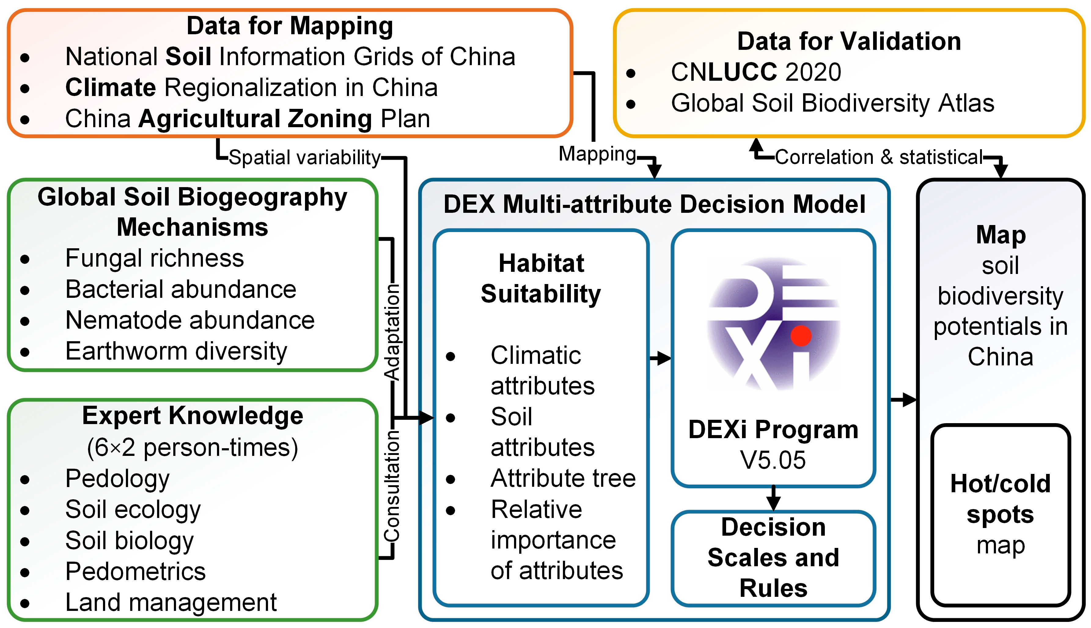
Taking China’s land area as the study area, we constructed a DEX multi-attribute decision model based on the presumed impact of abiotic factors such as soil and climate on soil biota. It was used to indirectly assess and map the national SBP based on the habitat suitability for fungi, bacteria, nematodes, and earthworms in the topsoil. Then, the spatial pattern of the mapped SBP was quantitatively described using spatial statistics, with the agricultural region as the unit. Finally, the validation of the results was discussed in terms of SBP differences among different agricultural land types and comparison with the Global Soil Biodiversity Atlas (Figure 1).
2.2. Study Area
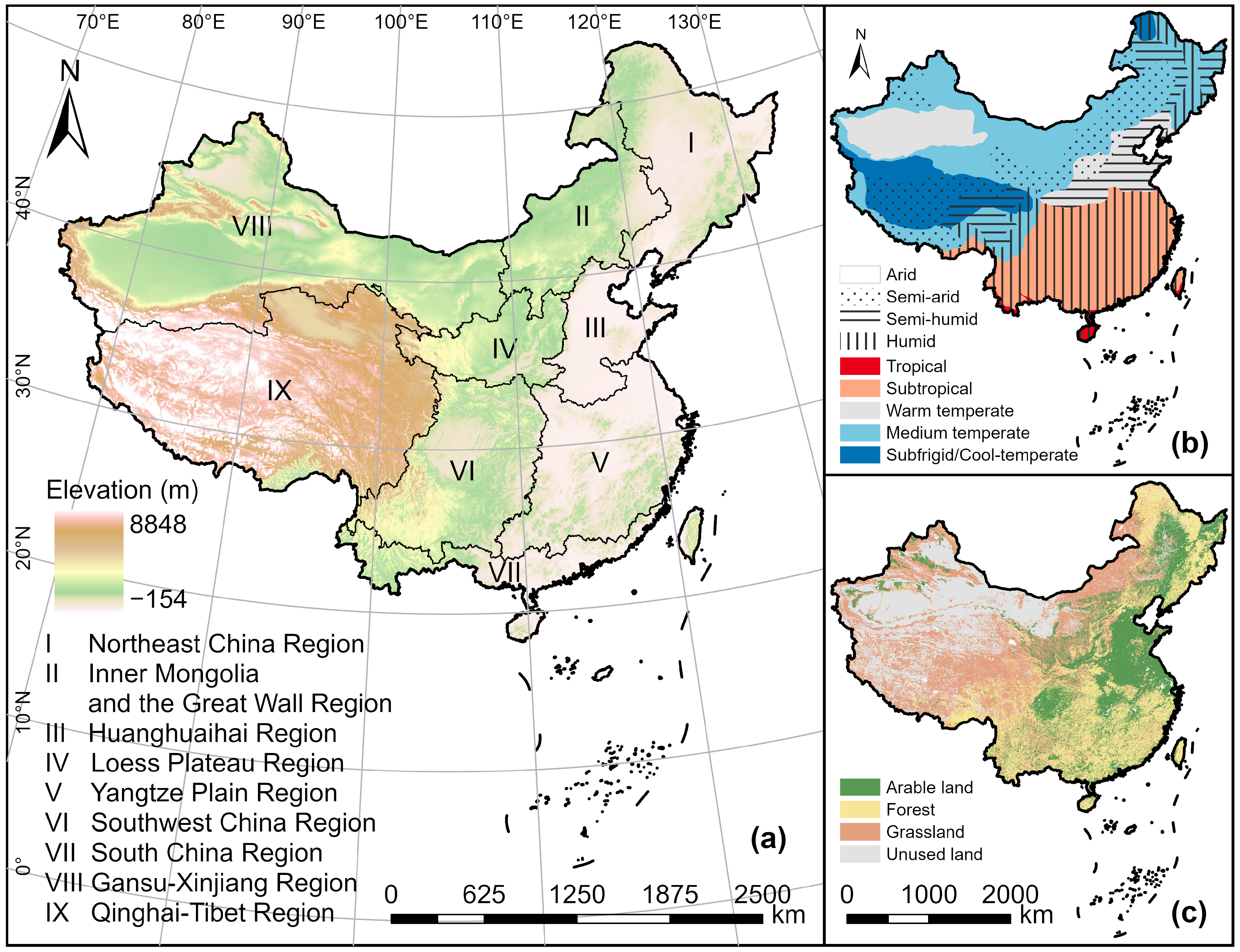
China is located on the east coast of the Eurasian continent and on the west coast of the Pacific Ocean (Figure 2a). Its topography is generally high in the west and low in the east, with a three-stage distribution. Nationwide, the five basic topographies are mountain (33.3%), plateau (26.0%), basin (18.8%), plain (12.0%), and hills (9.9%) in order of area share.
China’s climate ranges from tropical monsoons, subtropical monsoons, and temperate monsoons in the east to temperate continental arid climates in the northwest, all the way to alpine climates on the Tibetan Plateau [42] (Figure 2b). Compared with other places at the same latitude, China has low temperatures in winter and high temperatures in summer, with a large annual temperature difference.
China’s land area covers 9.6 × 10⁶ km2. Among them, there are 1279 × 103 km2 of arable land, nearly two-thirds of which is located north of the Qinling–Huaihe Line; 2841 × 103 km2 of forest, mainly in areas with annual precipitation of 400 mm or more; and 2645 × 103 km2 of grassland, mainly in Tibet, Inner Mongolia, Xinjiang, Qinghai, Gansu, and Sichuan provinces [41] (Figure 2c). According to the distribution characteristics of agricultural resources, the country is divided into nine agricultural regions and 38 agricultural subregions [40] (Figure 2a).
2.3. Data Source and Preprocessing
Six soil attributes in 1-km resolution gridded maps were accessed from the National Soil Information Grids of China [31]: pH, SOC, total nitrogen (total N), total phosphorus (total P), cation exchange capacity (CEC), and USDA textural classes (texture). The C/N ratio was calculated from SOC and total N. These data were available for 0–5–15–30 cm depths. For all soil data, those values that deviate more than three standard deviations from the mean were regarded as outliers and excluded. Additionally, the soil type data of the World Reference Base for Soil Resources (WRB) were obtained from the Harmonized World Soil Database version 2.0 [33].
Climate attribute data were accessed from the Climate Regionalization in China for 1981–2010 [42]. It is the latest scheme of climate regionalization in China, which integrally reveals the regional differentiation of climate and describes climate characteristics at the regional scale. Based on this scheme, our study divides China into five temperature zones, including subfrigid/cool-temperate, medium temperate, warm temperate, subtropical, and tropical zones, and four arid/humid regions, including humid, semi-humid, semi-arid, and arid regions (Figure 2b). It was gridded into a 1-km grid in accordance with the soil attribute data.
With respect to land use/land cover data for the interpretation of the evaluation results, a 100-m resolution gridded map of arable land, forest, and high (>50%)-medium (20–50%)-low (5–20%)-coverage grassland in 2020 (Figure 2c) was accessed from China’s Multi-period Land Use/Land Cover Remote Sensing Monitoring Dataset (CNLUCC) [41]. It was also gridded in accordance with the soil attribute data.
2.4. Construction of the DEX Multi-Attribute Decision Model
The DEX multi-attribute decision model is a subjective evaluation model that first deconstructs a complex problem and then makes a stepwise decision on a single problem based on a priori knowledge to achieve the evaluation objective [35,36,43]. It simplifies the complex problem and fuzzifies the hierarchy of indicator values to meet our two needs: (1) knowledge-based evaluation of SBP; and (2) discretization of indicator values to focus on significant rather than subtle changes in the habitat of soil biota, thus avoiding information redundancy caused by the sensitivity of soil biota. DEX modeling was implemented in the DEXi 5.05 program [44].
2.4.1. Indicator Soil Biota and Their Diversity Drivers
Due to the abundant availability of data on the geographic distribution of soil fungi, bacteria, nematodes, and earthworms, they serve as subjects for current global-scale soil biogeography research [23,24,25,26,27,28,45]. These studies provide a comprehensive understanding of these taxa, including their geographic distribution and habitat characteristics. Consequently, these four taxa were chosen as indicator soil biota to describe soil habitat suitability and to link SBP. They comprise three functional groups [46]: (1) As essential chemical engineers, fungi and bacteria are responsible for the chemical processes at the first level of the food web. It has been observed that fungi respond to soil environmental changes in a complete and significant gradient manner [11]. Bacteria are sensitive to soil management actions and are integrative—that is, they provide adequate coverage across a relatively wide range of environmental variables such as soil types, climate, and crop sequence [39,47,48]. (2) Nematodes, as biological regulators, are present in high abundance and richness, and their relative or absolute abundance provides valuable information on ecosystem diversity and stability [49,50]. (3) Earthworms are the most frequently used indicator species among ecosystem engineers and are highly relevant for structure formation, bioturbation, and related soil functions [51]. They were also widely used in European national or regional soil biodiversity monitoring networks [52].
The main drivers of the diversity (richness and abundance) of four soil taxa at the global scale were summarized in Table 1, with soil and climate being the two most important common drivers. The information provided by the different studies varies: firstly, those on fungi focused on diversity and richness, those on bacteria and nematodes on abundance, and the one on earthworms on diversity; secondly, the specific indicators of the drivers differ, and the driving forces were presented quantitatively or qualitatively in various forms such as numbers, graphs and text; thirdly, the main habitats of the four soil taxa are different, as reflected in the soil depths that these studies focused on, i.e., 0–5 cm for fungi and bacteria, 0–15 cm for nematodes, and 0–30 cm for earthworms; finally, there may be conflicts between studies, e.g., Tedersoo et al. [23] found the overall richness of soil fungi increased towards the equator, while in the analysis of Větrovský et al. [45], fungal diversity is concentrated at high latitudes. Before constructing the DEX model, this information needs to be manually interpreted and adapted.
2.4.2. Attribute Tree and the Relative Importance of Attributes
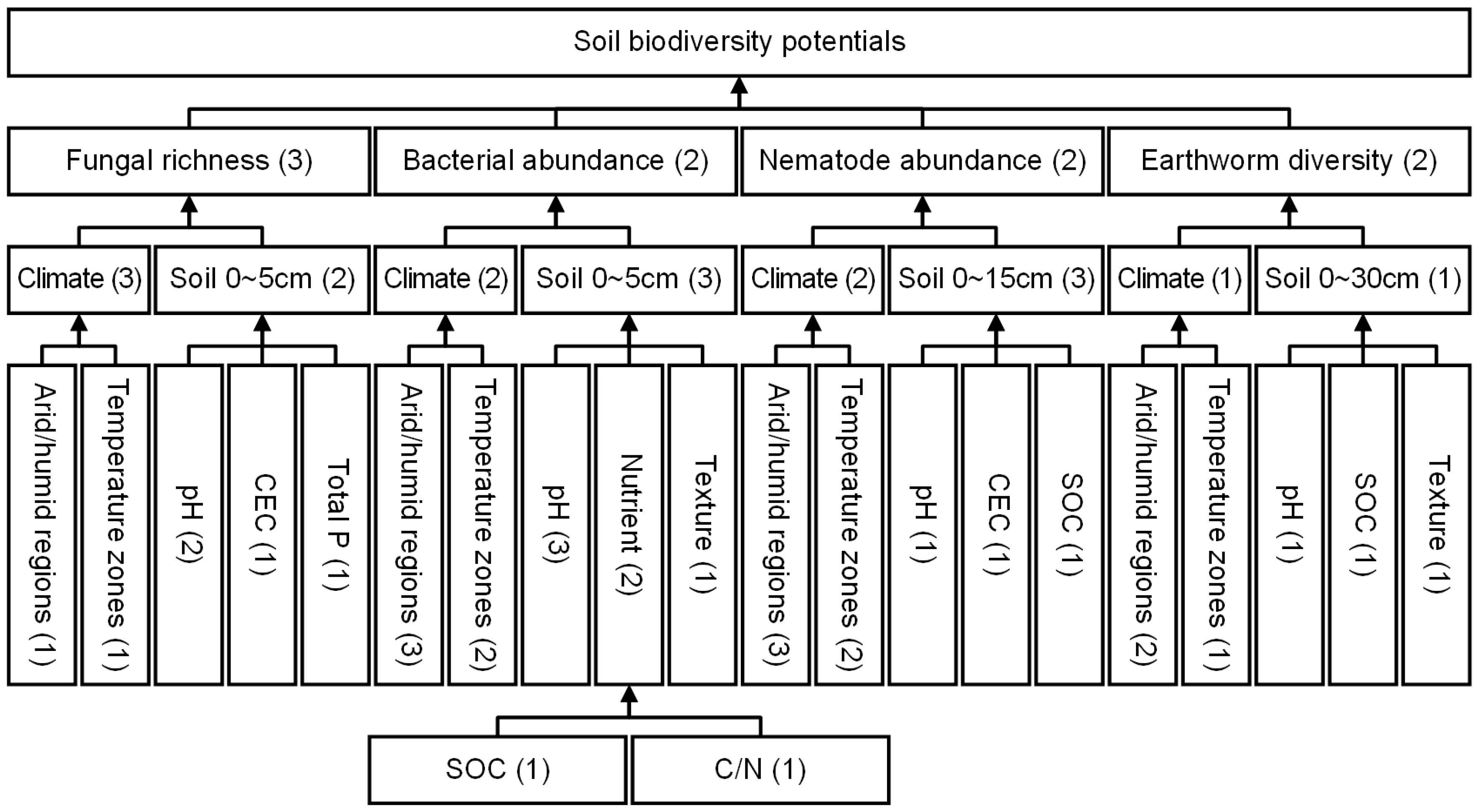
The first step in constructing the DEX model is to build an attribute tree. The attribute tree (Figure 3) for mapping SBP was built based on the adapted global-scale biogeographic research results (Table 1) and the DEXi Program Guidelines [53]. SBP was represented by four level I attributes: fungal richness, bacterial abundance, nematode abundance, and earthworm diversity. The four level I attributes were indicated by two level II habitat attributes, namely climate and soil. Considering data availability and operability, temperature zones and arid/humid regions were selected as two level III attributes characterizing climate. Soil pH, SOC, CEC, texture, total P, and C/N ratio were selected as the level III attributes characterizing soil.
As part of the biogeographic study (Table 1), the relative importance of each driver was also estimated. Each sibling attribute was assigned an importance score of 3, 2, or 1, respectively, with 3 being the highest and 1 being the lowest. Therefore, in the case of pairwise comparison, there are four relative importance relationships: 3:2, 3:1, 2:1, and 1:1 in the local sibling nodes. For example, the relative importance of the four level I attributes under SBP was set to 3, 2, 2, and 2, respectively; the relative importance of the two level II attributes, soil and climate, for the level I attribute, bacterial abundance, was set to 3 and 2, respectively; and so on. These relative importance scores would be converted proportionally into weights and used as parameters for developing the decision rules.
2.4.3. Attributes’ Scales
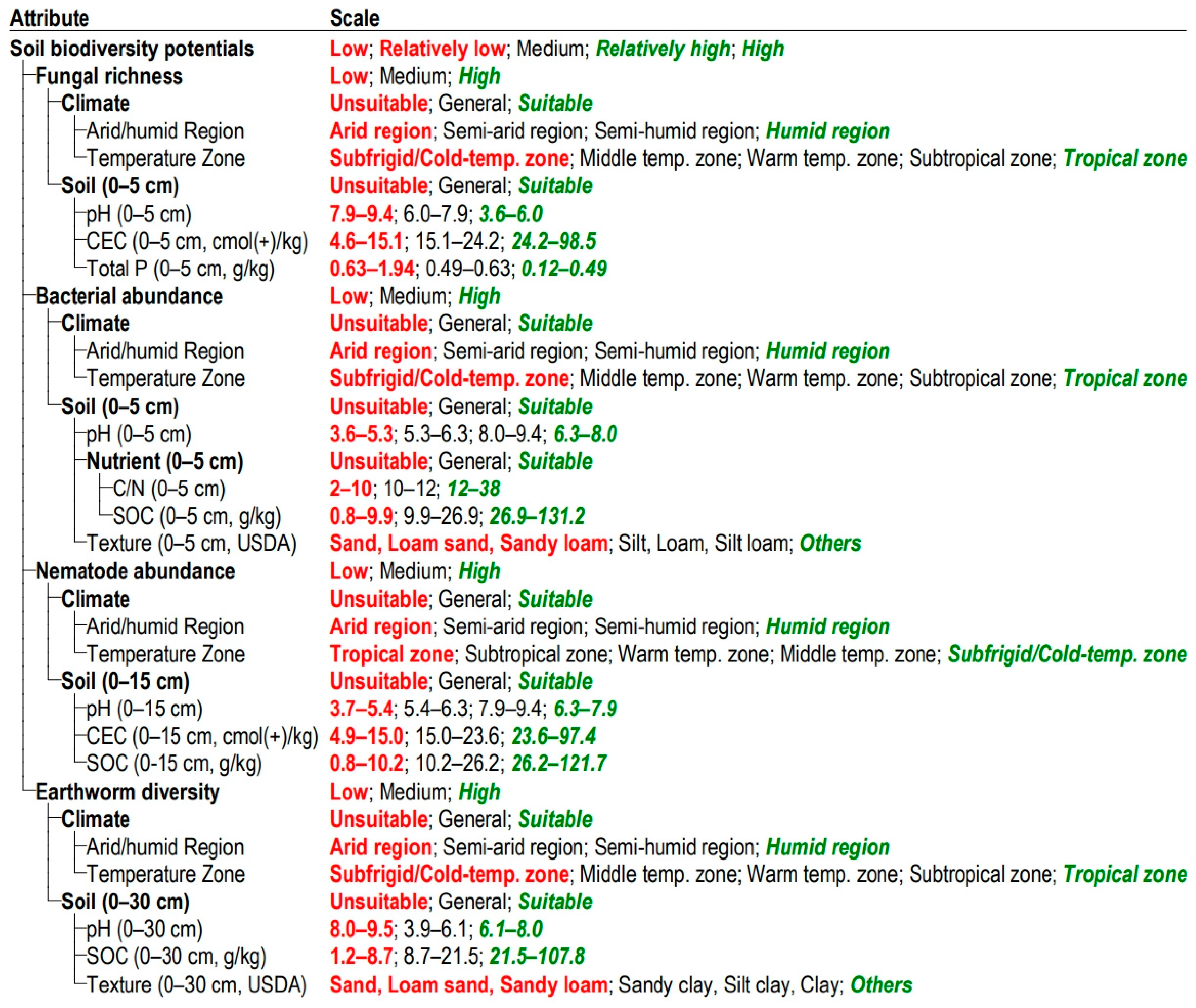
In the second step, the four types of soil biodiversity (richness or abundance) indicated in the above attribute tree (Figure 3) were classified into three to five grades from high to low; soil and climate attributes were classified into three grades from habitat suitable to unsuitable (Figure 4). In the DEX model, the grades of attributes are generated by the aggregation decision of the grades of their lower-level attributes. Therefore, the scales of the lowest-level attributes need to be determined first. For our study, we used the literature listed in Table 1 as the theoretical basis, combined with the spatial differentiation of these attributes in China.
Nominal attributes such as climate arid/humid regions, temperate zones, and soil texture were directly mapped to habitat-suitable, normal, and unsuitable grades with their original categories. For instance, in climate-arid/humid regions for earthworms, the humid region is suitable, the semi-humid region and semi-arid regions are normal, and the arid region is unsuitable. Moreover, numerical attributes were reclassified into three to four numerical intervals by the Geometrical Interval classification method in ArcGIS Pro, which ensures that each class range has approximately the same number of values and that the change between intervals is fairly consistent. These intervals were then mapped to the three grades of habitat suitability according to membership function types such as positive linear, negative linear, or kurtosis. For example, the higher SOC content is better for nematodes, so this relationship is a positive linear function. Specifically, an SOC content of 26.2 to 121.7 g/kg is considered suitable, 10.2 to 26.2 g/kg is normal, and 0.8 to 10.2 g/kg is unsuitable. Each attribute grade is a partition of that attribute value, confirming the completeness of the DEX model.
2.4.4. Expert Consultation for Model Optimization
The quality of the DEX model depends on the quality of the knowledge applied in modeling. In the process of forming the above attribute tree and its scales (Figure 4), six independent experts in pedology, soil ecology, soil biology, pedometrics, and land management were invited to consult on (1) the relative importance of attributes and (2) the scales of soil biological habitat suitability attributes. Multiple rounds of consultation were conducted to reach consensus.
Comments from the six invited experts covered all ten modules consulted and focused mainly on soil fungi, bacteria, and earthworms and less on nematodes (Table 2). Integrating 44 comments from all experts improved the DEX model.
2.4.5. Decision Rules
Each node of the DEX attribute tree has an independent decision rule that relies only on the next-level attributes to make a level-by-level decision. The definition of decision rules follows four principles: (1) If all the attributes at the next-level node are suitable, this node is suitable or high. (2) If all the attributes at the next-level node are normal, this node is normal or medium. (3) If all the attributes at the next-level node are unsuitable, this node is unsuitable or low. (4) Based on the above three principles, other cases are determined by the weight of the attribute, which is converted proportionally from the relative importance score in the DEXi 5.05 program [44] (Table 3).
2.5. Attribute Mapping
In ArcGIS Pro, the raster values of the bottom attributes were reclassified into three grades: suitable, normal, and unsuitable, according to the defined scales. Then, the Map Algebra expression of the Raster Calculator tool was used to map the national SBP step-by-step according to the decision rule. The map’s accuracy depends on the resolution of the soil raster data, which is 1 km here.
2.6. Spatial Analysis
First, the average SBP of China’s nine agricultural regions and 38 agricultural subregions was counted. Then, the Global Moran’s I was calculated to measure the spatial autocorrelation of national SBP based on the location and mean SBP values of each agricultural region, revealing whether the national SBP pattern was clustered, discrete, or random. If the z-score or p-value indicates statistical significance, a positive Global Moran’s I value indicates a clustering trend, and a negative value indicates a discrete trend. The Global Moran’s I value is calculated according to Cliff and Ord [54]:
where n is the number of spatial units indexed by i and j, x is the variable of interest, wi,j is the spatial weight between the spatial units i and j, and .
The z-score is computed as:
where .
Further, the Getis-Ord Gi* statistic was calculated to show the spatial clustering of higher SBP (hot spots) and lower SBP (cold spots) with statistical significance, thus identifying the focal areas. If the Gi* statistic of the spatial unit is statistically significant, the higher the positive Gi* statistic, the more significant the clustering of high SBP (hot spots), and the lower the negative Gi* statistic, the more significant the clustering of low SBP (cold spots). The Gi* statistic is calculated following Getis and Ord [55] and Ord and Getis [56]:
where n is the number of spatial units indexed by i and j, x is the variable of interest, S is the standard deviation of all x, and wi,j is the spatial weight between the spatial units i and j.
These spatial analyses were implemented using the Zonal Statistics, Spatial Autocorrelation (Global Moran’s I), and Hot Spot Analysis (Getis-Ord Gi*) tools in ArcGIS Pro 3.1.3.
3. Results
3.1. The Decision Rules of the DEX Multi-Attribute Decision Model
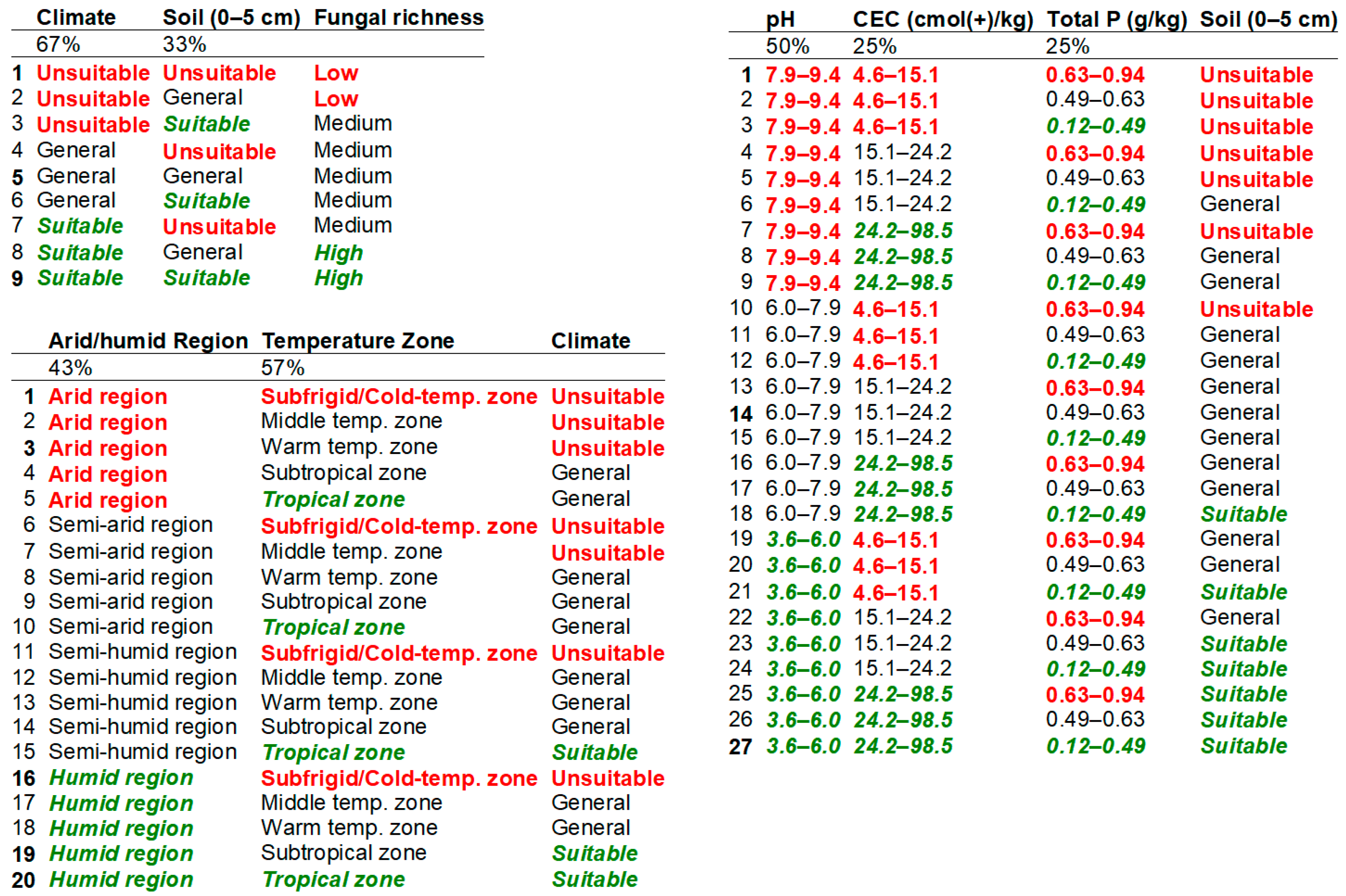
After initializing the DEX model and expert consultation, all 332 final decision rules were generated, which are shown in the Supplementary Material. The monotonicity of each utility function was verified by checking the “Use scale orders” box in the Function Editor of the DEXi program. Here, Figure 5 excerpts show the 56 decision rules for soil fungal richness. It consists of three levels and demonstrates a step-by-step decision-making process following the attribute tree and the four decision principles described in Section 2.4.5.
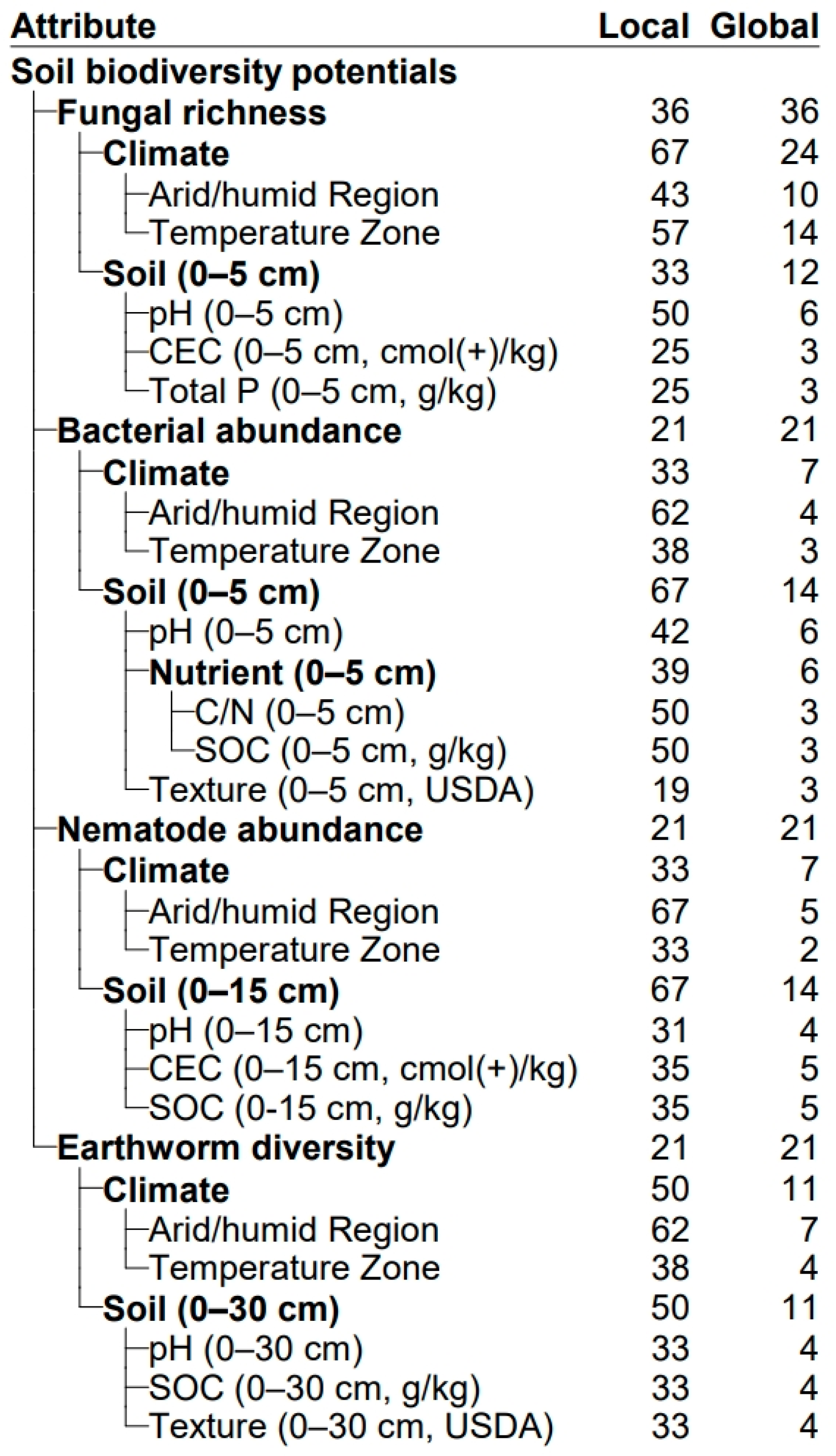
The vital parameters supporting the formation of these decision rules are shown in Figure 6, where the most important ones are the local weights, converted from the attributes’ relative importance, which represent the contribution (%) of the corresponding attribute in every individual decision process, and the global weights, which reflect the attributes’ weights (%) in the whole process. Among the bottom attributes at the global level, the arid/humid regions (26%) are the most important climate attribute, followed by temperature zones (23%); ignoring different topsoil depths, the contribution of soil attributes is pH (20%), SOC (12%), CEC (8%), texture (7%), total P (3%) and C/N (3%), in that order; soil attributes (51%) are almost as important as climate attributes (49%).
3.2. Habitat Suitability Maps of Four Soil Taxa in China
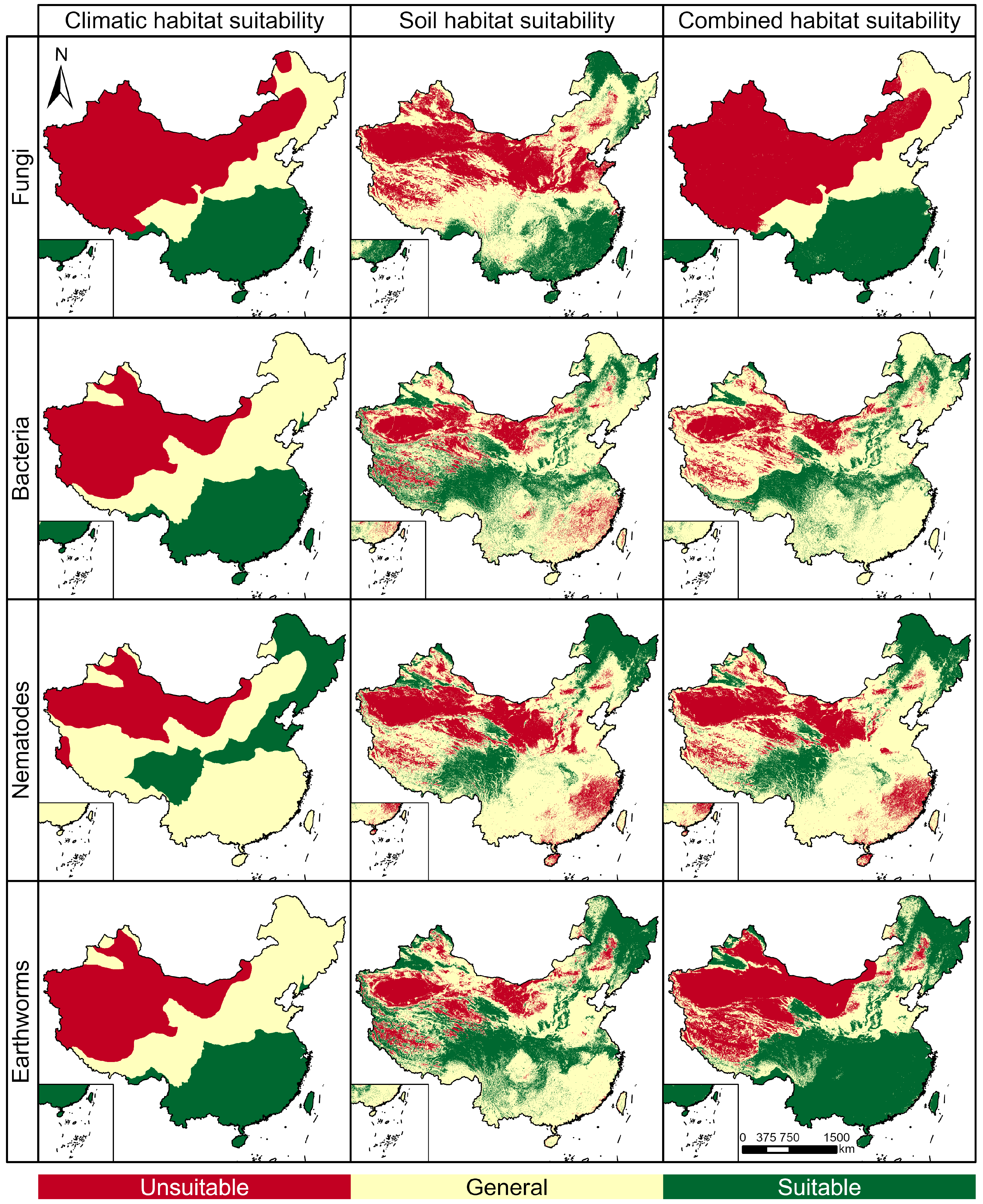
Climatic habitat suitability, soil habitat suitability, and combined climate and soil habitat suitability for soil fungi, bacteria, nematodes, and earthworms were mapped separately in the decision-making process for mapping national SBP, as shown in Figure 7. In terms of climatic suitability, bacteria and earthworms have the same spatial pattern; they and fungi show decreasing suitability from the southern warm-humid areas to the northwestern cold-arid areas; nematodes have high suitability in humid and semi-humid temperate areas, and on this axis, decreasing to the north and south, with the lowest in the northwestern cold-arid areas. In terms of soil suitability, the spatial patterns of the four soil taxa differed significantly, but the distribution law of soil suitability was not apparent due to the complex spatial heterogeneity and combined effects of soil attributes. In terms of combined climate and soil suitability, the spatial patterns of the four taxa are also different as affected by soils. The spatial mismatch between climate and soil suitability makes significant differences between the soil suitability and the combined climate and soil suitability of fungi, bacteria, and earthworms. Such as the soil conditions (low pH, high CEC) in the Greater and Lesser Khingan Mountains and the Changbai Mountains are suitable for fungi, but the cold climate limits their habitat; the warm–humid climate of the Southeast China Hills improves the poor soil conditions (coarse texture, low SOC, and pH), which are not suitable for bacteria and earthworms.
3.3. Map of Soil Biodiversity Potentials in China
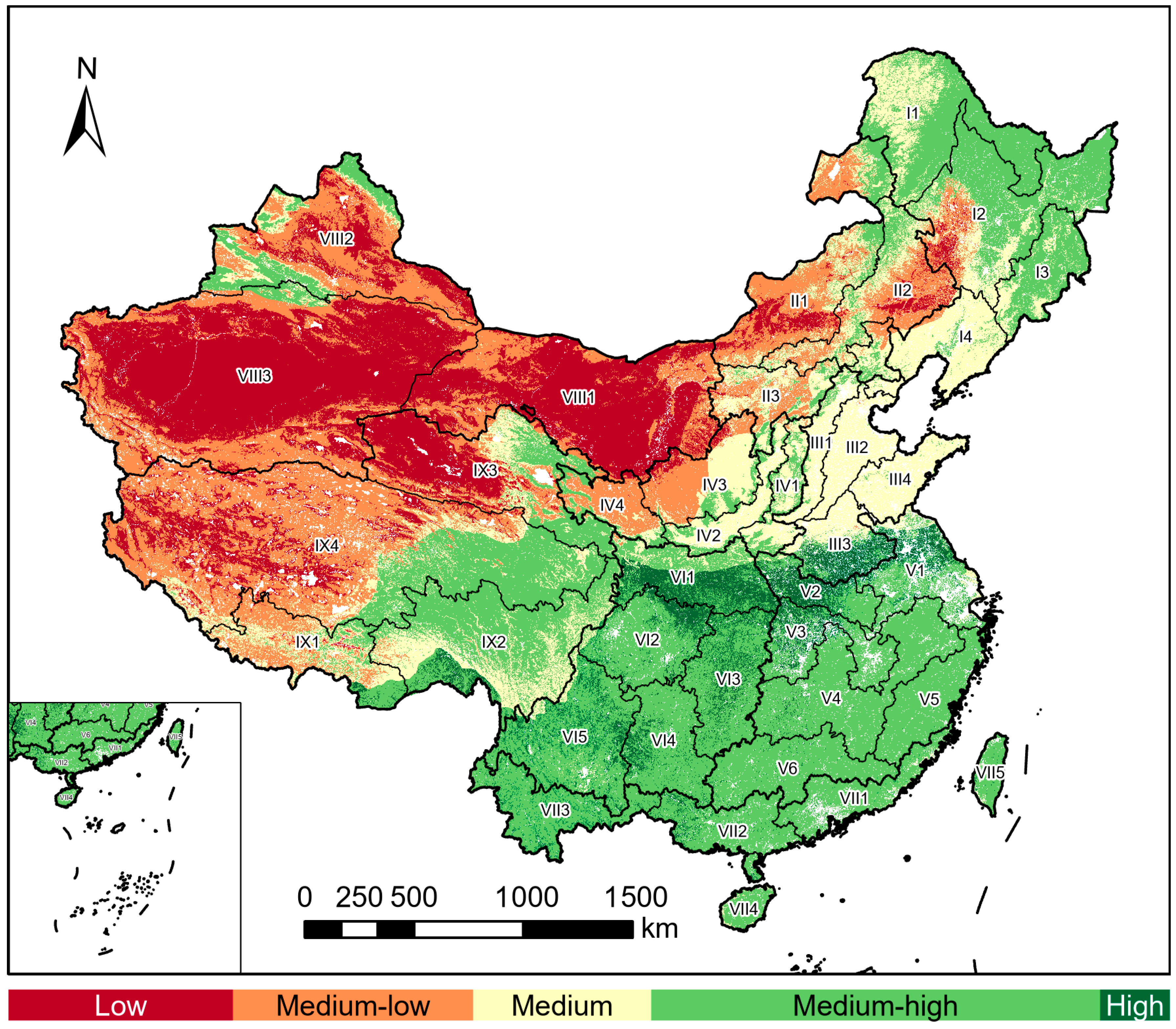
A whole-area SBP map was generated by integrating the above maps into the DEX model. Then, the raster of arable land, forest, grassland, and unused land was extracted to print a nationwide non-construction land SBP map with a total coverage area of 8,929,899 km2 (Figure 8). As a result, the national SBP was classified into five grades: low (1,767,379 km2, 19.8% of the area), medium-low (1,894,493 km2, 21.2%), medium (1,426,606 km2, 16.0%), medium-high (3,435,667 km2, 38.5%), and high (405,754 km2, 4.5%), with the scores corresponding to 1, 2, 3, 4, and 5. The national average SBP score is 2.87, considered medium SBP.
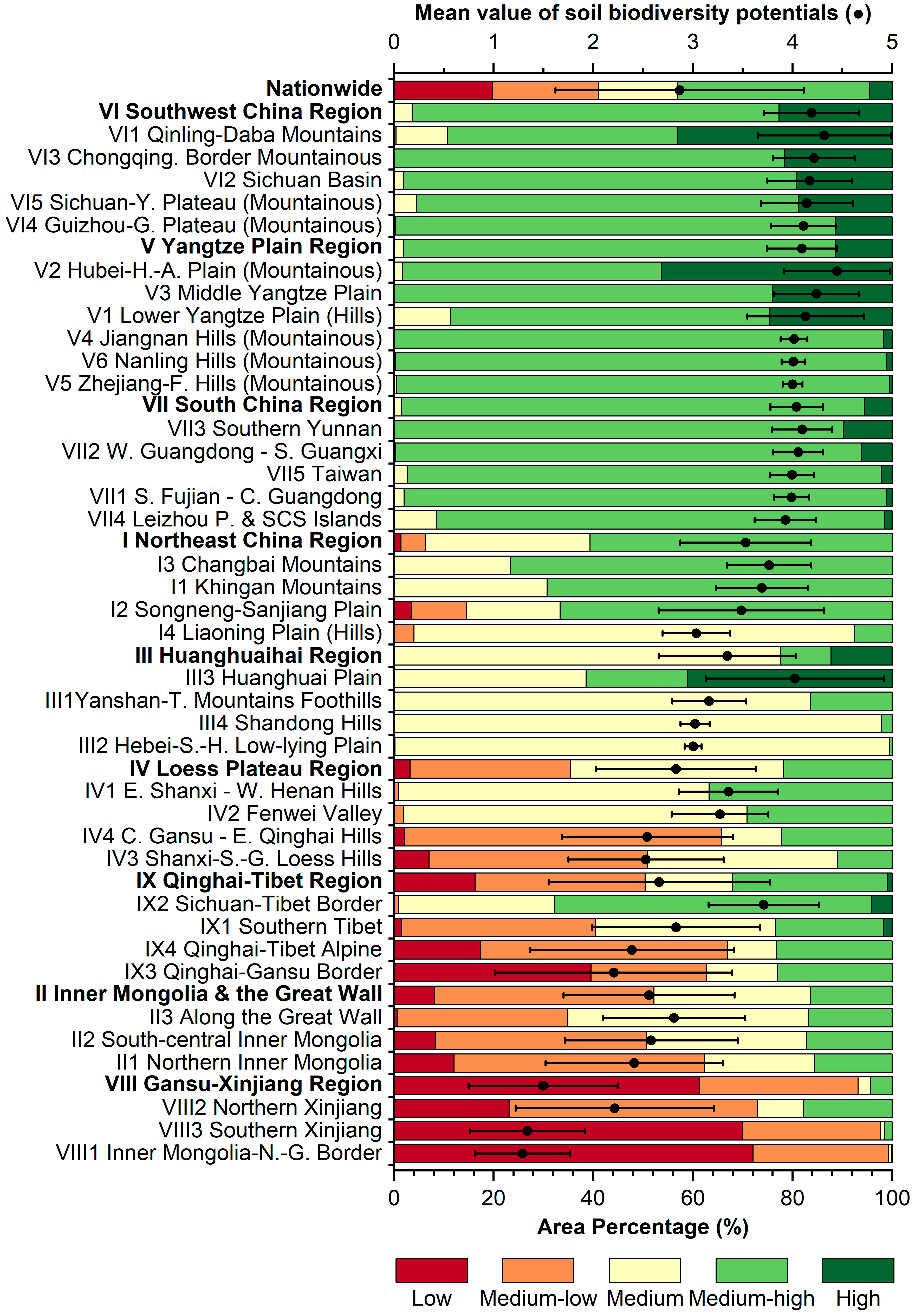
According to the statistics of agricultural regions (Figure 9), the average SBP of agricultural regions from high to low is: China Region (4.19), Yangtze Plain Region (4.09), South China Region (4.04), Northeast China Region (3.53), Huanghuaihai Region (3.35), Loess Plateau Region (2.83), Qinghai-Tibet Region (2.66), Inner Mongolia and the Great Wall Region (2.56), and Gansu–Xinjiang Region (1.50). Among them, the Southwest China, Yangtze Plain, South China, Northeast China, and Huanghuaihai regions score above the national average and have less spatial variation within regions, with a total area of 3,539,421 km2, accounting for 39.6% nationwide. In contrast, Loess Plateau, Qinghai–Tibet, Inner Mongolia and the Great Wall, and Gansu-Xinjiang regions are lower than the national average and have greater spatial variation within regions, with a total area of 5,389,603 km2, accounting for 60.4% nationwide. In general, the SBP of agricultural areas shows the distribution pattern of the Hu Line, i.e., the SBP of the area east of the Hu Line scores above the national average, and the area west of the Hu Line is lower than the national average.
The distribution of SBP in agricultural regions across the country is shown in Table 4. The high SBP areas are mainly distributed in the Southwest China, Yangtze Plain, Huanghuaihai, Qinghai–Tibet, and South China regions. The medium-high SBP areas are mainly distributed in the Qinghai–Tibet, Yangtze Plain, Northeast China, Southwest China, South China, and Gansu–Xinjiang regions. The medium SBP areas are mainly distributed in Qinghai-Tibet, Northeast China, Huanghuaihai, Inner Mongolia and the Great Wall, Loess Plateau, and Gansu–Xinjiang regions. The medium-low-SBP areas are mainly distributed in the Qinghai–Tibet, Gansu–Xinjiang, Inner Mongolia and the Great Wall, Loess Plateau, and Northeast China regions. The low-SBP areas are mainly distributed in the Gansu–Xinjiang and Qinghai–Tibet regions. Overall, the distribution of high SBP, low SBP, and medium-low SBP areas is generally clustered, while the medium-high SBP and medium SBP areas are relatively discrete and distributed across all agricultural subregions.
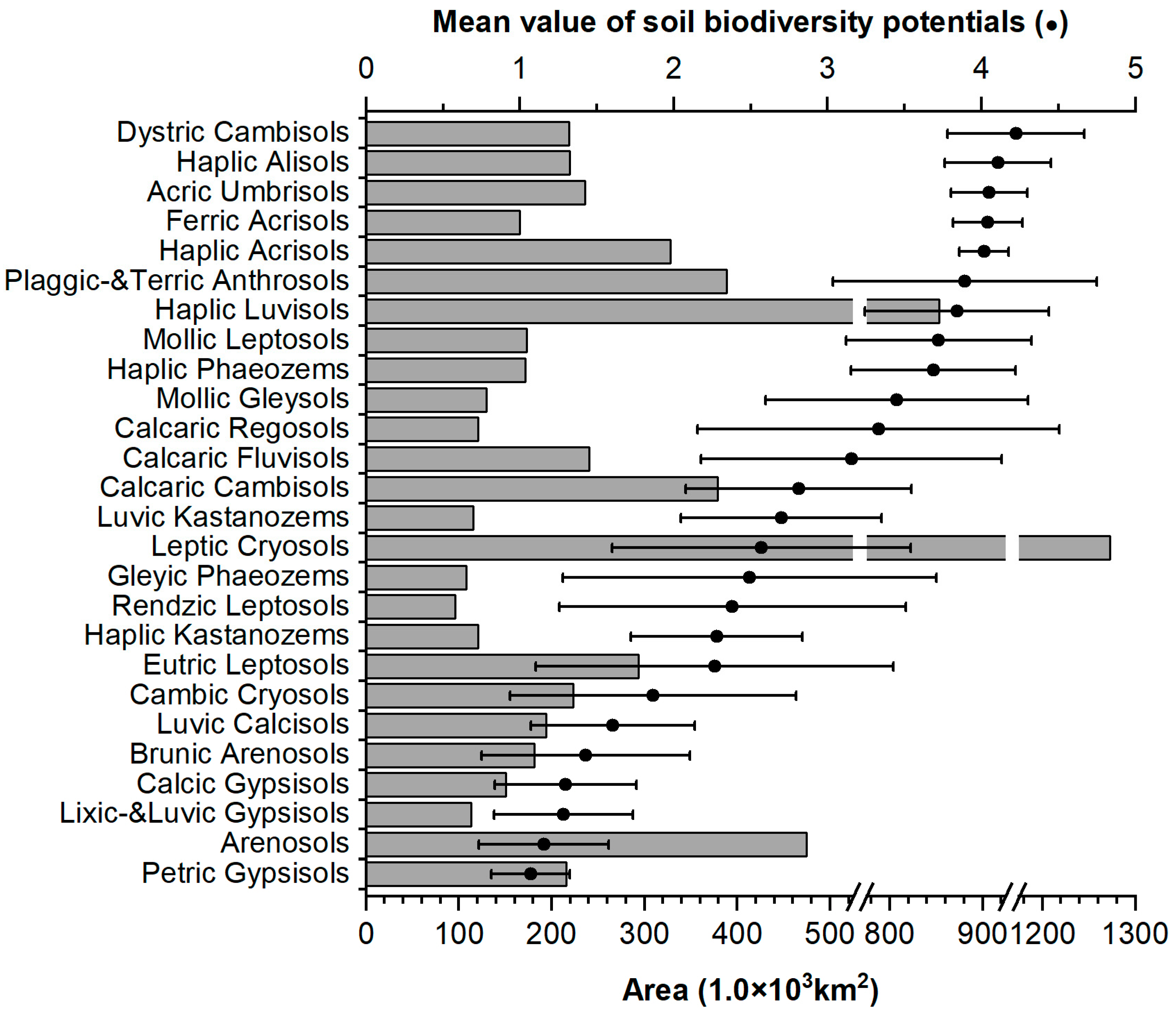
In terms of soil types (Figure 10), among the seven WRB Reference Soil Groups (RSGs) that cover more than 5% nationwide, the SBP ranges from high to low as follows: Acrisols, Luvisols, and Cambisols; Leptosols and Cryosols; Arenosols and Gypsisols. This sequence reflects various influences, primarily driven by climate, as evidenced by the stark contrast between Acrisols occurring in warm-humid areas and Arenosols and Gypsisols in arid regions. Secondly, soil physicochemical properties, such as Luvisols covered by forests, have favorable physical characteristics such as porosity and aeration; the widespread Cambisols possess medium texture, good structural stability, high porosity, excellent water retention capacity, and effective internal drainage, as well as neutral to weakly acid soil reactions, satisfactory chemical fertility, and active soil fauna. There are also cold environments and strongly dissected topography influenced by altitude, as seen in Leptosols and Cryosols.
3.4. Spatial Pattern Characteristics and Priority Areas of Soil Biodiversity Potentials in China
The Global Moran’s I statistics for the mean SBP scores of agricultural subregions showed a Moran’s I value of 0.725 > 0 for the national SBP and a z-score of 6.03 > +2.58 with a 99% confidence level. This indicates a significant, strong positive spatial autocorrelation (i.e., clustering of similar values) for the nationwide non-construction land SBP map (Figure 8). This is in accordance with the innate spatial autocorrelation of soil and climate properties.
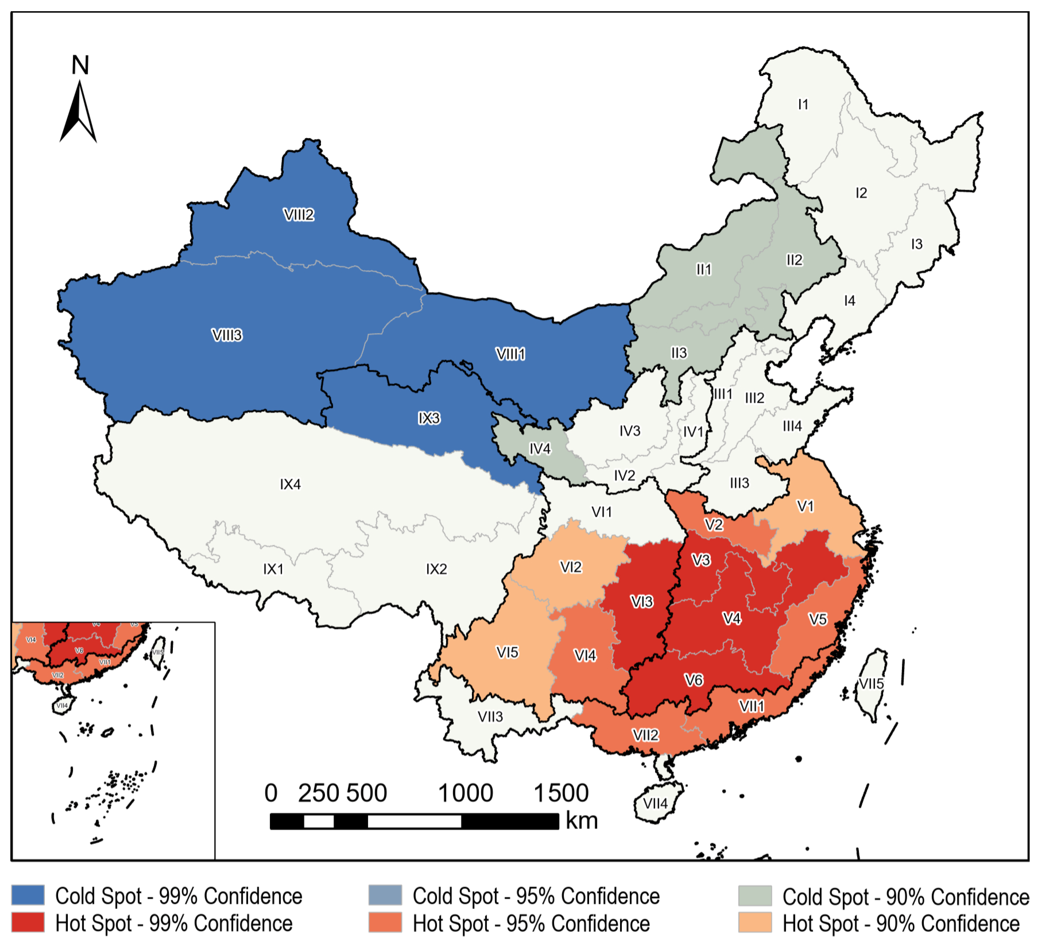
Further, the significant spatial clusters of higher SBP (hot spots) and lower SBP (cold spots) are shown in Figure 11 by the Getis-Ord Gi* statistic. At the 95% confidence level, the SBP hot spot area covers 1,338,040 km2 and accounts for 15.0% nationwide, while the SBP cold spot has an area of 2,566,618 km2 and accounts for 28.7% nationwide, which is almost twice the size of the hot spot area. Table 5 shows the natural conditions and agricultural characteristics of these areas.
4. Verification
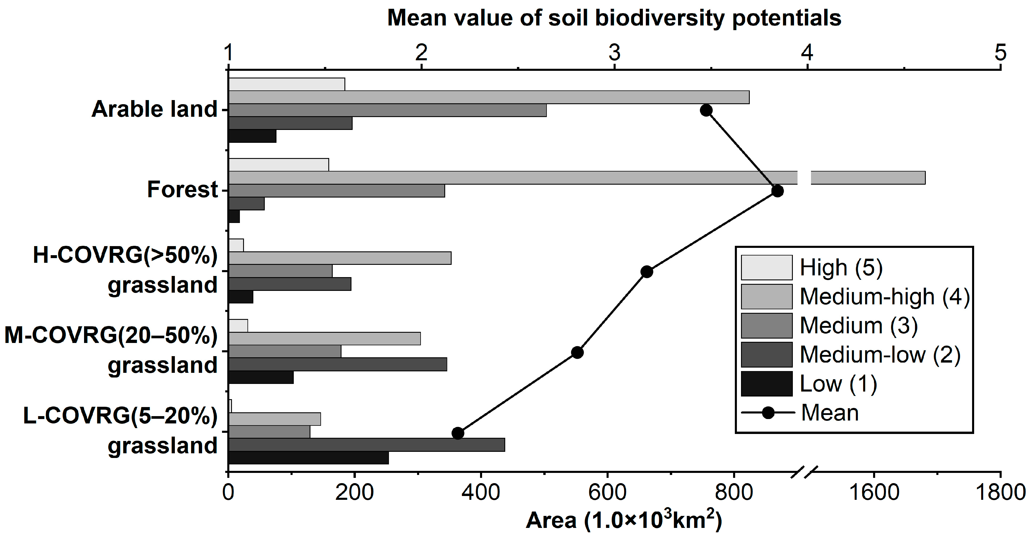
The commonly used “measured vs. simulated” validation approach is not practical here because of the lack of comparable soil biodiversity survey data over this vast area. So, two indirect validations were applied. First, by raster overlay analysis and one-way ANOVA, the mapped SBP was counted by five land use/land cover types, such as arable land, forest, and high/medium/low coverage grassland. Differences in SBP between land types are expected to be consistent with the general knowledge of soil biology research. As shown in Figure 12, the SBP of five land types is significantly different at the 0.05 level. Their mean values are between 2.19~3.84, with the highest in forest (3.84), followed by arable land (3.47) and high (>50%)-coverage grassland (3.17), and the lowest in medium-low (≤50%)-coverage grassland (2.19–2.81). Considering the apparent distribution differences between cropland and grassland, this SBP/land-types sequence generally reflects the general principle that lower land use intensity and less soil disturbance lead to higher soil biodiversity [57,58,59,60,61,62,63,64]. From this perspective, the evaluation result was considered reasonable.
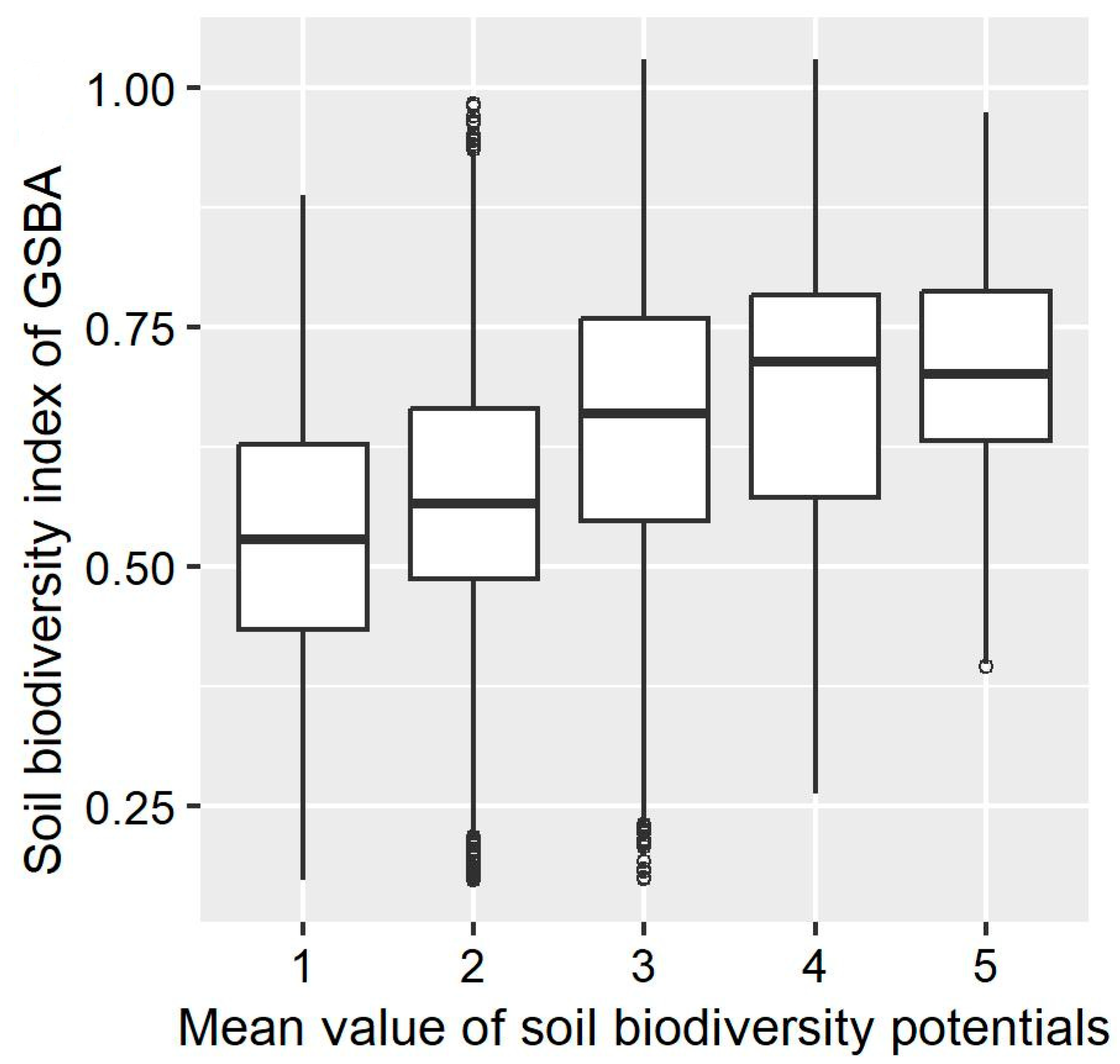
The mapped SBP was then compared with similar work covering China. Here the Global Soil Biodiversity Atlas [16] was selected, and the Spearman’s rank correlation revealed its correlation with the mapped SBP. A significant positive correlation would corroborate the concept of the SBP. Of course, there is a possibility that both maps are “overall” wrong, but this likelihood decreases as more data and knowledge contributing to the conceptual soil biodiversity model become available [20]. Therefore, if both maps exhibit a positive correlation, they provide mutual support for their validity. The analysis showed a Spearman’s rank correlation coefficient of 0.50 between the two maps, indicating a moderately positive correlation (Figure 13). A strong positive correlation could not be achieved. However, a possible explanation is that the Global Soil Biodiversity Atlas, as an exploratory global-scale result, represents a much coarser spatial resolution compared to our study.
5. Discussion
5.1. New Knowledge in Soil Biogeography Develops the Soil Biodiversity Assessment at Large Spatial Scales
Knowledge about soil biodiversity is central to mapping SBP. The mechanisms affecting soil biodiversity are complex and are being elucidated from multiple perspectives and scales, from climate change to land use, and from field trials to global geography. Due to the extreme complexity of interacting mechanisms acting under vastly different site conditions, there are no clear relationships between a limited number of site characteristics and soil biodiversity. This leads to contradictory observations even when many influencing factors are the same or in the same geographical region. This is reflected not only in publications, such as the discussion of tropical and temperate patterns of earthworm diversity by Phillips et al. [28] and James et al. [65], but also in our consultations with experienced experts. This is a major issue for SBP mapping.
Soil biogeography aims to study the ecological distributions of soil biota’s diversity, community composition, and functional traits across space and time, from regional to global scales [66]. The relationship between soil biodiversity and environmental covariates is a core research element. Recently published global-scale soil biogeography results emerge as the most robust information available. Although the derived global-scale laws of soil biodiversity differentiation are inherently coarse-grained and may not fully capture more nuanced regional conditions, they have a higher possibility of balancing rationality and universality, offering a versatile framework for understanding and application. Taking advantage of this, we present a national-scale SBP mapping solution based on understanding the relationship between soil biodiversity and site conditions using available soil and climate data, clarifying the systematic basis for selecting indicators and determining their weights from a relatively objective perspective.
Indeed, with decades of research accumulated in Europe on soil assessment about biodiversity [67], a solid knowledge base has been built: from monitoring networks and their indicators [59,68,69,70,71], potential risk estimation [72], to expert system-based [15,16,20,21,22] and survey data-driven [20,73,74,75,76] soil biodiversity mapping. However, we still have great difficulty adjusting complex indicator parameters when applying previous methods to China, unless we organize an extensive expert system or already have a wealth of survey data. This is a great challenge for China, which has nine agricultural regions. SBP mapping based on soil biogeography and the adaptable DEX model is a potential choice that is universal and easily transferable to other areas.
We highlight that knowledge gaps remain regarding the habitat suitability of soil biota and the scale of the impact of climatic factors on soil biodiversity. The method we used to reclassify numerical attributes by a combination of data spatial variability and membership function type is applicable here, but the reclassification results would be more interpretable and general if they could be based on the exact suitable habitat for soil biota. These issues rely on a stronger data and knowledge base. So, we call for China’s Third National Soil Survey (2022–2025) to pay attention to the national-scale soil biological survey based on soil species sampling, covering major climatic regions, topographic conditions, and land use types, as a way to advance soil biogeography research further.
5.2. Soil Biogeography Knowledge Applied to the DEX Multi-Attribute Decision Model
We have clarified the rationality of using global-scale soil biogeography findings for SBP mapping. Growing global-scale research is labor-intensive and complicated, sometimes conflicting with scientists’ opinions. There are also differences in the processes and expressions of studies on different soil taxa. We assigned an importance score (3, 2, or 1) to fuzzily normalize information on indicator weights from different studies according to numerical, graphical, or textual descriptions in the literature—the information is diverse. Numerical attributes, mainly soil attributes, were discretized into grades based on spatial variability. Both steps are intended to circumvent the uncertainty caused by soil biota’s sensitivity and improve the assessment’s error tolerance. Although, inevitably, such an approach and the accompanying nonlinear decision rules of the DEX model sacrifice sensitivity compared to dimensionless scoring functions. In addition, knowledge conflicts are always in the process of knowledge-based assessment, mainly between literature and expert comments on the relative importance of attributes. We followed the principle of larger-scale prioritization—leaning on large-scale meta-analysis evidence, followed by second-round consultation with experts. As a result, knowledge from multiple sources of literature and experts was aggregated through the DEX model.
Climate is an important driver for the spatial differentiation of global soil biodiversity. We have integrated climate attributes into the DEX model and graded them using standard climate regionalization, which has more meteorological significance and interpretability than geostatistical classification methods such as geometrical interval. But this allows the climate suitability maps to present some climate regionalization boundaries that also appear in the SBP map. These boundaries in the SBP map reflect the possible overly strong role of climate attributes in the DEX model for national SBP. Climate is also a critical soil-forming factor [77,78], and differences in soil properties may reflect differences in climatic conditions as well. The trade-off of climatic factors in national-scale SBP mapping needs to be supported by further theoretical understanding [79].
5.3. Application of the Map of Soil Biodiversity Potentials at the National Scale
Mapping the national SBP on a kilometer grid is an effective way to understand the patterns of soil habitat function. Since soil biodiversity over large areas is not easy to measure consistently from field sampling [80], nor is it realistic to predict accurately from current knowledge. The large-scale soil function mapping aims to serve the macro-layout of soil resource utilization and conservation, in contrast to the field soil function evaluation for local management strategies. The agricultural regional SBP map and hot/cold spots map would provide a reference for China’s Third National Soil Survey (2022–2025) to identify priority areas for soil biological survey and also provide nationally comparable benchmark parameters for soil biodiversity indicators in land evaluation.
Moreover, this study provides a space-for-time substitution [81] perspective to examine the relationship between SBP, soil types, and land use. The Second Level RSGs covering more than 3.0 × 10⁶ km2 nationwide are Haplic Acrisols, Plaggic-&Terric Anthrosols, Haplic Luvisols, Calcaric Cambisols, Leptic Cryosols, and Arenosols, which have significantly lower SBP in turn. Meanwhile, their primary productivity also decreases in turn, confirming the synergy between soil habitat function and production function. According to the pattern of SBP and land use, we suggest that:
- In the Yangtze Plain and Pearl River Delta, explore the symbiotic development of intensive agricultural production and biodiversity in densely populated areas;
- In the Jiangnan Hills and Southeast Coastal Hills, establish a long-term monitoring network of forest soil biodiversity to maintain a high level of soil biodiversity;
- In the Eastern Sichuan Hills and Guizhou–Guangxi Karst Hills, conduct SBP risk assessment on farmland to jointly conserve soil biodiversity;
- In the Gansu–Xinjiang Region and Qaidam Basin, given the low SBP baseline conditions in northwest arid areas, moderately cultivate native vegetation to prevent deterioration of the soil ecological environment.
5.4. Limitations
This methodology aims to reveal national patterns of soil habitat function by treating soil biodiversity potentials as the primary focus, particularly in the absence of extensive spatial data on soil biodiversity across large areas. As a multi-attribute decision approach, a solid foundation of scientific understanding, both from the literature and expert experience, is highly demanded. The understanding of the geographical distribution and habitat characteristics of soil organisms is still developing. Based on the current progress, this study selected soil fungi, bacteria, nematodes, and earthworms as indicator soil biota and could not synthesize species numbers across the tree of life, and the SBP assessment did not focus on both the richness and abundance—the complete components of the diversity concept—of each taxon. With the development of soil biogeography and the implementation of soil biological surveys, it is reasonable to expect this method to have a more solid theoretical foundation.
6. Conclusions
Mapping soil biodiversity potentials (SBP) is a practical way to uncover the national patterns of soil habitat function. It is essential for the sustainable management of soil resources. In this study, a DEX multi-attribute decision model was constructed by integrating the mechanisms of soil and climate factors on soil biota to characterize the distribution of SBP in China from the perspectives of topsoil fungi, bacteria, nematodes, and earthworm habitat suitability. The results indicate that the national SBP is at a moderate level. The SBP of the agricultural regions east of the Hu Line is higher than the national average, and the region west of the Hu Line is lower than the national average. The hotspot areas are located in the Yangtze Plain Region, the southeastern Southwest China Region, and the central-eastern South China Region, covering 15.0% nationwide, while the coldspot areas are located in the Gansu–Xinjiang Region and the northeastern Qinghai–Tibet Region, covering 28.7% nationwide. Soil (pH, SOC, CEC, texture, total P, and C/N) and climate (arid/humid regions, temperature zones) drive this SBP variation.
SBP mapping based on soil biogeography and the DEX model presented a general solution to describe the habitat function at a broad scale with environmental covariates data. It clarifies the systematic basis for the selection of indicators and determines the indicators and their weights from an objective perspective. This methodology is suitable for regions where soil biota is not surveyed and can also be used as a pre-survey for planning soil resource utilization and conservation. The scale effect of climatic factors is still being clarified here, pending further knowledge. With the development of soil biogeography and the implementation of soil biological surveys, a fine-resolution soil biodiversity map covering a wider area is expected.
Supplementary Materials
The following supporting information can be downloaded at: https://www.mdpi.com/article/10.3390/agronomy13112822/s1.
Author Contributions
Conceptualization, Q.Y. and K.W.; Investigation, Q.Y. and K.W.; Methodology, Q.Y., U.W. and F.L.; Resources, H.-J.V., F.L. and K.W.; Software, Q.Y.; Writing—original draft, Q.Y.; Writing—review and editing, U.W., H.-J.V. and Z.F. All authors have read and agreed to the published version of the manuscript.
Funding
This work was funded by the National Key R&D Program of China [No. 2018YFE0107000]; the National Natural Science Foundation of China [No. 42171261]; and the German Federal Ministry of Education and Research (BMBF) in the framework of the funding measure “Soil as a Sustainable Resource for the Bioeconomy—BonaRes”, project “BonaRes (Module B): BonaRes Centre for Soil Research, subproject A” [grant 031B1064A].
Data Availability Statement
The data presented in this study are available on request from the corresponding author.
Acknowledgments
We thank Huixin Li (Nanjing Agricultural University), Chi Zhang (South China Agricultural University), Huaizhi Tang (China Agricultural University), Minjie Yao (Fujian Agriculture and Forestry University), Songchao Chen (ZJU-Hangzhou Global Scientific and Technological Innovation Center), and Jialong Wu (Guangzhou Institute of Forestry and Landscape Architecture) who participated in the expert consultation for model optimization. We also thank the China Scholarship Council (File No. 202106400061) for supporting this study. And acknowledgement for the data support from “Soil SubCenter, National Earth System Science Data Center, National Science & Technology Infrastructure of China. (http://soil.geodata.cn (accessed on 8 March 2022))”.
Conflicts of Interest
The authors declare no conflict of interest.
References
- Shen, R.; Wang, C.; Sun, B. Soil related scientific and technological problems in implementing strategy of “Storing Grain in Land and Technology”. Bull. Chin. Acad. Sci. 2018, 33, 135–144. [Google Scholar] [CrossRef]
- Tang, H.; Sang, L.; Yun, W. China’s cultivated land balance policy implementation dilemma and direction of scientific and technological innovation. Bull. Chin. Acad. Sci. 2020, 35, 637–644. [Google Scholar] [CrossRef]
- Xu, M.; Lu, C.; Zhang, W.; Li, l.; Duan, Y. Situation of the quality of arable land in China and improvement strategy. Chin. J. Agric. Resour. Reg. Plan. 2016, 37, 8–14. [Google Scholar] [CrossRef]
- Zhou, J. Evolution of soil quality and sustainable use of soil resources in China. Bull. Chin. Acad. Sci. 2015, 30, 459–467. [Google Scholar] [CrossRef]
- Wu, K.; Yang, Q.; Zhao, R. A discussion on soil health assessment of arable land in China. Acta Pedol. Sin. 2021, 58, 537–544. [Google Scholar] [CrossRef]
- Helming, K.; Daedlow, K.; Paul, C.; Techen, A.-K.; Bartke, S.; Bartkowski, B.; Kaiser, D.; Wollschläger, U.; Vogel, H.-J. Managing soil functions for a sustainable bioeconomy—Assessment framework and state of the art. Land Degrad. Dev. 2018, 29, 3112–3126. [Google Scholar] [CrossRef]
- Vogel, H.J.; Bartke, S.; Daedlow, K.; Helming, K.; Kögel-Knabner, I.; Lang, B.; Rabot, E.; Russell, D.; Stößel, B.; Weller, U.; et al. A systemic approach for modeling soil functions. Soil 2018, 4, 83–92. [Google Scholar] [CrossRef]
- Schulte, R.P.O.; Creamer, R.E.; Donnellan, T.; Farrelly, N.; Fealy, R.; O’Donoghue, C.; O’hUallachain, D. Functional land management: A framework for managing soil-based ecosystem services for the sustainable intensification of agriculture. Environ. Sci. Policy 2014, 38, 45–58. [Google Scholar] [CrossRef]
- Bardgett, R.D.; van der Putten, W.H. Belowground biodiversity and ecosystem functioning. Nature 2014, 515, 505–511. [Google Scholar] [CrossRef]
- Lavelle, P.; Decaëns, T.; Aubert, M.; Barot, S.; Blouin, M.; Bureau, F.; Margerie, P.; Mora, P.; Rossi, J.P. Soil invertebrates and ecosystem services. Eur. J. Soil Biol. 2006, 42, S3–S15. [Google Scholar] [CrossRef]
- Wagg, C.; Bender, S.F.; Widmer, F.; van der Heijden, M.G.A. Soil biodiversity and soil community composition determine ecosystem multifunctionality. Proc. Natl. Acad. Sci. USA 2014, 111, 5266–5270. [Google Scholar] [CrossRef] [PubMed]
- Lehmann, J.; Bossio, D.A.; Kögel-Knabner, I.; Rillig, M.C. The concept and future prospects of soil health. Nat. Rev. Earth Environ. 2020, 1, 544–553. [Google Scholar] [CrossRef]
- McBratney, A.; Field, D.J.; Koch, A. The dimensions of soil security. Geoderma 2014, 213, 203–213. [Google Scholar] [CrossRef]
- Orgiazzi, A.; Panagos, P.; Fernández-Ugalde, O.; Wojda, P.; Labouyrie, M.; Ballabio, C.; Franco, A.; Pistocchi, A.; Montanarella, L.; Jones, A. LUCAS Soil Biodiversity and LUCAS Soil Pesticides, new tools for research and policy development. Eur. J. Soil Sci. 2022, 73, e13299. [Google Scholar] [CrossRef]
- Jeffery, S.; Gardi, C.; Jones, A.; Montanarella, L.; Marmo, L.; Miko, L.; Ritz, K.; Peres, G.; Römbke, J.; van der Putten, W.H. European Atlas of Soil Biodiversity; European Commission, Publications Office of the European Union: Luxembourg, 2010. [Google Scholar]
- Orgiazzi, A.; Bardgett, R.D.; Barrios, E.; Behan-Pelletier, V.; Briones, M.J.I.; Chotte, J.-L.; De Deyn, G.B.; Eggleton, P.; Fierer, N.; Fraser, T.; et al. Global Soil Biodiversity Atlas; European Commission, Publications Office of the European Union: Luxembourg, 2016. [Google Scholar]
- Greiner, L.; Keller, A.; Grêt-Regamey, A.; Papritz, A. Soil function assessment: Review of methods for quantifying the contributions of soils to ecosystem services. Land Use Policy 2017, 69, 224–237. [Google Scholar] [CrossRef]
- Vogel, H.J.; Eberhardt, E.; Franko, U.; Lang, B.; Liess, M.; Weller, U.; Wiesmeier, M.; Wollschlager, U. Quantitative evaluation of soil functions: Potential and state. Front. Environ. Sci. 2019, 7, 164. [Google Scholar] [CrossRef]
- Yang, Q.; Wu, K.; Feng, Z.; Zhao, R.; Zhang, X.; Li, X. Soil quality assessment on large spatial scales: Advancement and revelation. Acta Pedol. Sin. 2020, 57, 565–579. [Google Scholar] [CrossRef]
- Rutgers, M.; van Leeuwen, J.P.; Vrebos, D.; van Wijnen, H.J.; Schouten, T.; de Goede, R.G.M. Mapping soil biodiversity in Europe and the Netherlands. Soil Syst. 2019, 3, 39. [Google Scholar] [CrossRef]
- van Leeuwen, J.P.; Creamer, R.E.; Cluzeau, D.; Debeljak, M.; Gatti, F.; Henriksen, C.B.; Kuzmanovski, V.; Menta, C.; Pérès, G.; Picaud, C.; et al. Modeling of soil functions for assessing soil quality: Soil biodiversity and habitat provisioning. Front. Environ. Sci. 2019, 7, 113. [Google Scholar] [CrossRef]
- Aksoy, E.; Louwagie, G.; Gardi, C.; Gregor, M.; Schröder, C.; Löhnertz, M. Assessing soil biodiversity potentials in Europe. Sci. Total Environ. 2017, 589, 236–249. [Google Scholar] [CrossRef]
- Tedersoo, L.; Bahram, M.; Põlme, S.; Kõljalg, U.; Yorou, N.S.; Wijesundera, R.; Ruiz, L.V.; Vasco-Palacios, A.M.; Thu, P.Q.; Suija, A.; et al. Global diversity and geography of soil fungi. Science 2014, 346, 1256688. [Google Scholar] [CrossRef] [PubMed]
- Větrovský, T.; Morais, D.; Kohout, P.; Lepinay, C.; Algora, C.; Awokunle Hollá, S.; Bahnmann, B.D.; Bílohnědá, K.; Brabcová, V.; D’Alò, F.; et al. GlobalFungi, a global database of fungal occurrences from high-throughput-sequencing metabarcoding studies. Sci. Data 2020, 7, 228. [Google Scholar] [CrossRef] [PubMed]
- Delgado-Baquerizo, M.; Oliverio, A.M.; Brewer, T.E.; Benavent-González, A.; Eldridge, D.J.; Bardgett, R.D.; Maestre, F.T.; Singh, B.K.; Fierer, N. A global atlas of the dominant bacteria found in soil. Science 2018, 359, 320–325. [Google Scholar] [CrossRef]
- Van den Hoogen, J.; Geisen, S.; Routh, D.; Ferris, H.; Traunspurger, W.; Wardle, D.A.; de Goede, R.G.M.; Adams, B.J.; Ahmad, W.; Andriuzzi, W.S.; et al. Soil nematode abundance and functional group composition at a global scale. Nature 2019, 572, 194–198. [Google Scholar] [CrossRef] [PubMed]
- Van den Hoogen, J.; Geisen, S.; Wall, D.H.; Wardle, D.A.; Traunspurger, W.; de Goede, R.G.M.; Adams, B.J.; Ahmad, W.; Ferris, H.; Bardgett, R.D.; et al. A global database of soil nematode abundance and functional group composition. Sci. Data 2020, 7, 103. [Google Scholar] [CrossRef] [PubMed]
- Phillips, H.R.P.; Guerra, C.A.; Bartz, M.L.C.; Briones, M.J.I.; Brown, G.; Crowther, T.W.; Ferlian, O.; Gongalsky, K.B.; van den Hoogen, J.; Krebs, J.; et al. Global distribution of earthworm diversity. Science 2019, 366, 480–485. [Google Scholar] [CrossRef]
- Arrouays, D.; Grundy, M.G.; Hartemink, A.E.; Hempel, J.W.; Heuvelink, G.B.M.; Hong, S.Y.; Lagacherie, P.; Lelyk, G.; McBratney, A.B.; McKenzie, N.J.; et al. GlobalSoilMap: Toward a fine-resolution global grid of soil properties. Adv. Agron. 2014, 125, 93–134. [Google Scholar] [CrossRef]
- Chen, S.C.; Arrouays, D.; Leatitia Mulder, V.; Poggio, L.; Minasny, B.; Roudier, P.; Libohova, Z.; Lagacherie, P.; Shi, Z.; Hannam, J.; et al. Digital mapping of GlobalSoilMap soil properties at a broad scale: A review. Geoderma 2022, 409, 115567. [Google Scholar] [CrossRef]
- Liu, F.; Wu, H.Y.; Zhao, Y.G.; Li, D.; Yang, J.-L.; Song, X.; Shi, Z.; Zhu, A.X.; Zhang, G.-L. Mapping high resolution National Soil Information Grids of China. Sci. Bull. 2022, 67, 328–340. [Google Scholar] [CrossRef]
- Poggio, L.; de Sousa, L.M.; Batjes, N.H.; Heuvelink, G.B.M.; Kempen, B.; Ribeiro, E.; Rossiter, D. SoilGrids 2.0: Producing soil information for the globe with quantified spatial uncertainty. Soil 2021, 7, 217–240. [Google Scholar] [CrossRef]
- FAO; IIASA. Harmonized World Soil Database Version 2.0; FAO: Rome, Italy, 2023. [Google Scholar] [CrossRef]
- Köninger, J.; Panagos, P.; Jones, A.; Briones, M.J.I.; Orgiazzi, A. In defence of soil biodiversity: Towards an inclusive protection in the European Union. Biol. Conserv. 2022, 268, 109475. [Google Scholar] [CrossRef]
- Bohanec, M. DEX (Decision EXpert): A qualitative hierarchical multi-criteria method. In Multiple Criteria Decision Making: Techniques, Analysis and Applications; Kulkarni, A.J., Ed.; Springer: Singapore, 2022; pp. 39–78. [Google Scholar]
- Bohanec, M.; Žnidaržič, M.; Rajkovič, V.; Bratko, I.; Zupan, B. DEX methodology: Three decades of qualitative multi-attribute modeling. Informatica 2013, 37, 49–54. [Google Scholar]
- Bampa, F.; O’Sullivan, L.; Madena, K.; Sandén, T.; Spiegel, H.; Henriksen, C.B.; Ghaley, B.B.; Jones, A.; Staes, J.; Sturel, S.; et al. Harvesting European knowledge on soil functions and land management using multi-criteria decision analysis. Soil Use Manag. 2019, 35, 6–20. [Google Scholar] [CrossRef]
- Debeljak, M.; Trajanov, A.; Kuzmanovski, V.; Schröder, J.; Sandén, T.; Spiegel, H.; Wall, D.P.; Van de Broek, M.; Rutgers, M.; Bampa, F.; et al. A field-scale decision support system for assessment and management of soil functions. Front. Environ. Sci. 2019, 7, 115. [Google Scholar] [CrossRef]
- FAO; ITPS; GSBI; CBD; EC. State of Knowledge of Soil Biodiversity—Status, Challenges and Potentialities; FAO, ITPS, GSBI, CBD and EC: Rome, Italy, 2020. [Google Scholar]
- Nationwide Committee of Agricultural Regionalization. Comprehensive Agricultural Regionalization of China; China Agriculture Press: Beijing, China, 1981. [Google Scholar]
- Xu, X.; Liu, J.; Zhang, S.; Li, R.; Yan, C.; Wu, S. China’s Multi-Period Land Use/Land Cover Remote Sensing Monitoring Dataset (CNLUCC). 2018. Available online: https://www.resdc.cn/DOI/doi.aspx?DOIid=54 (accessed on 1 June 2021).
- Zheng, J.; Bian, J.; Ge, Q.; Hao, Z.; Yin, Y.; Liao, Y. The climate regionalization in China for 1981–2010. Chin. Sci. Bull. 2013, 58, 3088–3099. [Google Scholar] [CrossRef]
- Bohanec, M.; Rajkovič, V. Multi-attribute decision modeling: Industrial applications of DEX. Informatica 1999, 23, 487–491. [Google Scholar]
- Bohanec, M.; Rajkovič, V.; Jereb, E.; Rajkovič, U.; Vintar, Z. DEXi: A Program for Multi-Attribute Decision Making, Version 5.05. Available online: https://kt.ijs.si/MarkoBohanec/dexi.html (accessed on 1 June 2021).
- Větrovský, T.; Kohout, P.; Kopecký, M.; Machac, A.; Man, M.; Bahnmann, B.D.; Brabcová, V.; Choi, J.; Meszárošová, L.; Human, Z.R.; et al. A meta-analysis of global fungal distribution reveals climate-driven patterns. Nat. Commun. 2019, 10, 5142. [Google Scholar] [CrossRef]
- Turbé, A.; de Toni, A.; Benito, P.; Lavelle, P.; Lavelle, P.; Ruiz Camacho, N.; van Der Putten, W.H.; Labouze, E.; Mudgal, S. Soil Biodiversity: Functions, Threats and Tools for Policy Makers; HAL: Paris, France, 2010. [Google Scholar]
- Luan, L.; Jiang, Y.; Dini-Andreote, F.; Crowther, T.W.; Li, P.; Bahram, M.; Zheng, J.; Xu, Q.; Zhang, X.-X.; Sun, B. Integrating pH into the metabolic theory of ecology to predict bacterial diversity in soil. Proc. Natl. Acad. Sci. USA 2023, 120, e2207832120. [Google Scholar] [CrossRef]
- Xue, P.; Minasny, B.; McBratney, A.; Pino, V.; Fajardo, M.; Luo, Y. Distribution of soil bacteria involved in C cycling across extensive environmental and pedogenic gradients. Eur. J. Soil Sci. 2023, 74, e13337. [Google Scholar] [CrossRef]
- Luan, L.; Jiang, Y.; Cheng, M.; Dini-Andreote, F.; Sui, Y.; Xu, Q.; Geisen, S.; Sun, B. Organism body size structures the soil microbial and nematode community assembly at a continental and global scale. Nat. Commun. 2020, 11, 6406. [Google Scholar] [CrossRef]
- Stone, D.; Costa, D.; Daniell, T.J.; Mitchell, S.M.; Topp, C.F.E.; Griffiths, B.S. Using nematode communities to test a European scale soil biological monitoring programme for policy development. Appl. Soil Ecol. 2016, 97, 78–85. [Google Scholar] [CrossRef]
- Blouin, M.; Hodson, M.E.; Delgado, E.A.; Baker, G.; Brussaard, L.; Butt, K.R.; Dai, J.; Dendooven, L.; Peres, G.; Tondoh, J.E.; et al. A review of earthworm impact on soil function and ecosystem services. Eur. J. Soil Sci. 2013, 64, 161–182. [Google Scholar] [CrossRef]
- Pulleman, M.; Creamer, R.; Hamer, U.; Helder, J.; Pelosi, C.; Pérès, G.; Rutgers, M. Soil biodiversity, biological indicators and soil ecosystem services—An overview of European approaches. Curr. Opin. Environ. Sustain. 2012, 4, 529–538. [Google Scholar] [CrossRef]
- Bohanec, M. DEXi: Program for Multi-Attribute Decision Making, User’s Manual; IJS Report DP-13100; Jožef Stefan Institute: Ljubljana, Slovenia, 2021. [Google Scholar]
- Cliff, A.D.; Ord, J.K. Spatial Autocorrelation; Pion: London, UK, 1973. [Google Scholar]
- Getis, A.; Ord, J.K. The analysis of spatial association by use of distance statistics. Geogr. Anal. 1992, 24, 189–206. [Google Scholar] [CrossRef]
- Ord, J.K.; Getis, A. Local spatial autocorrelation statistics: Distributional Issues and an application. Geogr. Anal. 1995, 27, 286–306. [Google Scholar] [CrossRef]
- Briones, M.J.I.; Schmidt, O. Conventional tillage decreases the abundance and biomass of earthworms and alters their community structure in a global meta-analysis. Glob. Chang. Biol. 2017, 23, 4396–4419. [Google Scholar] [CrossRef]
- Creamer, R.E.; Hannula, S.E.; Leeuwen, J.P.V.; Stone, D.; Rutgers, M.; Schmelz, R.M.; Ruiter, P.C.d.; Hendriksen, N.B.; Bolger, T.; Bouffaud, M.L.; et al. Ecological network analysis reveals the inter-connection between soil biodiversity and ecosystem function as affected by land use across Europe. Appl. Soil Ecol. 2016, 97, 112–124. [Google Scholar] [CrossRef]
- Rutgers, M.; Schouten, A.J.; Bloem, J.; Van Eekeren, N.; De Goede, R.G.M.; Jagersop Akkerhuis, G.A.J.M.; Van der Wal, A.; Mulder, C.; Brussaard, L.; Breure, A.M. Biological measurements in a nationwide soil monitoring network. Eur. J. Soil Sci. 2009, 60, 820–832. [Google Scholar] [CrossRef]
- Siebert, J.; Ciobanu, M.; Schädler, M.; Eisenhauer, N. Climate change and land use induce functional shifts in soil nematode communities. Oecologia 2020, 192, 281–294. [Google Scholar] [CrossRef]
- Spurgeon, D.J.; Keith, A.M.; Schmidt, O.; Lammertsma, D.R.; Faber, J.H. Land-use and land-management change: Relationships with earthworm and fungi communities and soil structural properties. BMC Ecol. 2013, 13, 46. [Google Scholar] [CrossRef]
- Tsiafouli, M.A.; Thébault, E.; Sgardelis, S.P.; de Ruiter, P.C.; van der Putten, W.H.; Birkhofer, K.; Hemerik, L.; de Vries, F.T.; Bardgett, R.D.; Brady, M.V.; et al. Intensive agriculture reduces soil biodiversity across Europe. Glob. Chang. Biol. 2015, 21, 973–985. [Google Scholar] [CrossRef] [PubMed]
- Van Leeuwen, J.P.; Djukic, I.; Bloem, J.; Lehtinen, T.; Hemerik, L.; de Ruiter, P.C.; Lair, G.J. Effects of land use on soil microbial biomass, activity and community structure at different soil depths in the Danube floodplain. Eur. J. Soil Biol. 2017, 79, 14–20. [Google Scholar] [CrossRef]
- Xue, P.; Minasny, B.; McBratney, A.B. Land-use affects soil microbial co-occurrence networks and their putative functions. Appl. Soil Ecol. 2022, 169, 104184. [Google Scholar] [CrossRef]
- James, S.W.; Csuzdi, C.; Chang, C.-H.; Aspe, N.M.; Jiménez, J.J.; Feijoo, A.; Blouin, M.; Lavelle, P. Comment on “Global distribution of earthworm diversity”. Science 2021, 371, eabe4629. [Google Scholar] [CrossRef]
- Chu, H.Y.; Gao, G.-F.; Ma, Y.Y.; Fan, K.; Delgado-Baquerizo, M. Soil microbial biogeography in a changing world: Recent advances and future perspectives. mSystems 2020, 5, e00803–e00819. [Google Scholar] [CrossRef]
- Lemanceau, P.; Creamer, R.; Griffiths, B.S. Soil biodiversity and ecosystem functions across Europe: A transect covering variations in bio-geographical zones, land use and soil properties. Appl. Soil Ecol. 2016, 97, 1–2. [Google Scholar] [CrossRef]
- Griffiths, B.S.; Rombke, J.; Schmelz, R.M.; Scheffczyk, A.; Faber, J.H.; Bloem, J.; Peres, G.; Cluzeau, D.; Chabbi, A.; Suhadolc, M.; et al. Selecting cost effective and policy-relevant biological indicators for European monitoring of soil biodiversity and ecosystem function. Ecol. Indic. 2016, 69, 213–223. [Google Scholar] [CrossRef]
- Ritz, K.; Black, H.I.J.; Campbell, C.D.; Harris, J.A.; Wood, C. Selecting biological indicators for monitoring soils: A framework for balancing scientific and technical opinion to assist policy development. Ecol. Indic. 2009, 9, 1212–1221. [Google Scholar] [CrossRef]
- Stone, D.; Ritz, K.; Griffiths, B.G.; Orgiazzi, A.; Creamer, R.E. Selection of biological indicators appropriate for European soil monitoring. Appl. Soil Ecol. 2016, 97, 12–22. [Google Scholar] [CrossRef]
- van Leeuwen, J.P.; Saby, N.P.A.; Jones, A.; Louwagie, G.; Micheli, E.; Rutgers, M.; Schulte, R.P.O.; Spiegel, H.; Toth, G.; Creamer, R.E. Gap assessment in current soil monitoring networks across Europe for measuring soil functions. Environ. Res. Lett. 2017, 12, 124007. [Google Scholar] [CrossRef]
- Gardi, C.; Jeffery, S.; Saltelli, A. An estimate of potential threats levels to soil biodiversity in EU. Glob. Chang. Biol. 2013, 19, 1538–1548. [Google Scholar] [CrossRef] [PubMed]
- Dequiedt, S.; Saby, N.P.A.; Lelievre, M.; Jolivet, C.; Thioulouse, J.; Toutain, B.; Arrouays, D.; Bispo, A.; Lemanceau, P.; Ranjard, L. Biogeographical patterns of soil molecular microbial biomass as influenced by soil characteristics and management. Glob. Ecol. Biogeogr. 2011, 20, 641–652. [Google Scholar] [CrossRef]
- Griffiths, R.I.; Thomson, B.C.; Plassart, P.; Gweon, H.S.; Stone, D.; Creamer, R.E.; Lemanceau, P.; Bailey, M.J. Mapping and validating predictions of soil bacterial biodiversity using European and national scale datasets. Appl. Soil Ecol. 2016, 97, 61–68. [Google Scholar] [CrossRef]
- Rutgers, M.; Orgiazzi, A.; Gardi, C.; Römbke, J.; Jänsch, S.; Keith, A.M.; Neilson, R.; Boag, B.; Schmidt, O.; Murchie, A.K.; et al. Mapping earthworm communities in Europe. Appl. Soil Ecol. 2016, 97, 98–111. [Google Scholar] [CrossRef]
- Terrat, S.; Horrigue, W.; Dequietd, S.; Saby, N.P.A.; Lelièvre, M.; Nowak, V.; Tripied, J.; Régnier, T.; Jolivet, C.; Arrouays, D.; et al. Mapping and predictive variations of soil bacterial richness across France. PLoS ONE 2017, 12, e0186766. [Google Scholar] [CrossRef]
- Jenny, H. Factors of soil formation. Soil Sci. 1941, 52, 415. [Google Scholar] [CrossRef]
- McBratney, A.B.; Mendonça Santos, M.L.; Minasny, B. On digital soil mapping. Geoderma 2003, 117, 3–52. [Google Scholar] [CrossRef]
- Liang, Y.T.; Xiao, X.; Nuccio, E.E.; Yuan, M.; Zhang, N.; Xue, K.; Cohan, F.M.; Zhou, J.; Sun, B. Differentiation strategies of soil rare and abundant microbial taxa in response to changing climatic regimes. Environ. Microbiol. 2020, 22, 1327–1340. [Google Scholar] [CrossRef]
- Cameron, E.K.; Martins, I.S.; Lavelle, P.; Mathieu, J.; Tedersoo, L.; Gottschall, F.; Guerra, C.A.; Hines, J.; Patoine, G.; Siebert, J.; et al. Global gaps in soil biodiversity data. Nat. Ecol. Evol. 2018, 2, 1042–1043. [Google Scholar] [CrossRef]
- Pickett, S.T.A. Space-for-time substitution as an alternative to long-term studies. In Long-Term Studies in Ecology: Approaches and Alternatives; Springer: New York, NY, USA, 1989; pp. 110–135. [Google Scholar]
Figure 1.
Technical roadmap for assessing soil biodiversity potentials in China based on the DEX multi-attribute decision model.
Figure 1.
Technical roadmap for assessing soil biodiversity potentials in China based on the DEX multi-attribute decision model.

Figure 2.
China’s location, topography, agricultural regions (a), climate (b), and land use/land cover (c) (data accessed from Nationwide Committee of Agricultural Regionalization [40]; Xu et al. [41]; Zheng et al. [42]).

Figure 3.
Attribute tree of the DEX multi-attribute decision model for assessing soil biodiversity potentials in China. The values 3, 2, and 1 are the relative importance scores of the attributes, with 3 being the highest and 1 being the lowest.
Figure 3.
Attribute tree of the DEX multi-attribute decision model for assessing soil biodiversity potentials in China. The values 3, 2, and 1 are the relative importance scores of the attributes, with 3 being the highest and 1 being the lowest.

Figure 4.
Attribute trees and their scales of the DEX multi-attribute decision model for assessing soil biodiversity potentials in China. The green interval or type means positive (suitable/high), black means normal, and red means negative (unsuitable/low).
Figure 4.
Attribute trees and their scales of the DEX multi-attribute decision model for assessing soil biodiversity potentials in China. The green interval or type means positive (suitable/high), black means normal, and red means negative (unsuitable/low).

Figure 5.
Decision rules of the DEX multi-attribute decision model for assessing soil biodiversity potentials in China (Soil fungal richness section). The green interval or type means positive (suitable/high), black means normal, and red means negative (unsuitable/low). The percentages represent the local weight of the attributes.

Figure 6.
Attributes’ weights of the DEX multi-attribute decision model for assessing soil biodiversity potentials in China.
Figure 6.
Attributes’ weights of the DEX multi-attribute decision model for assessing soil biodiversity potentials in China.

Figure 7.
Habitat suitability maps of soil fungi, bacteria, nematodes, and earthworms in China.

Figure 8.
Map of soil biodiversity potentials in China. The region code is the same as in Table 4.
Figure 8.
Map of soil biodiversity potentials in China. The region code is the same as in Table 4.

Figure 9.
Mean values of soil biodiversity potentials and proportions of potential areas at various grades by agricultural regions and subregions of China.
Figure 9.
Mean values of soil biodiversity potentials and proportions of potential areas at various grades by agricultural regions and subregions of China.

Figure 10.
Coverage area and soil biodiversity potentials of the WRB Second Level Reference Soil Groups (covering >1% nationwide) in China.
Figure 10.
Coverage area and soil biodiversity potentials of the WRB Second Level Reference Soil Groups (covering >1% nationwide) in China.

Figure 11.
Hot and cold spots map of soil biodiversity potentials in China. The region code is the same as in Table 4 and Table 5.

Figure 12.
Differences in soil biodiversity potentials of arable land, forest, and high-medium-low coverage grassland in China.
Figure 12.
Differences in soil biodiversity potentials of arable land, forest, and high-medium-low coverage grassland in China.

Figure 13.
Box plot of the soil biodiversity potentials and the soil biodiversity index of Global Soil Biodiversity Atlas.
Figure 13.
Box plot of the soil biodiversity potentials and the soil biodiversity index of Global Soil Biodiversity Atlas.


Table 1.
Drivers of biodiversity of soil fungi, bacteria, nematodes, and earthworms at the global scale.
Table 1.
Drivers of biodiversity of soil fungi, bacteria, nematodes, and earthworms at the global scale.
| Types | Primary Drivers | Other Main Drivers | References |
|---|---|---|---|
| Fungal richness (0–5 cm) | Climate (Latitude, Mean annual precipitation) | Soil (pH, Calcium (CEC), Phosphorus) | [23] |
| Fungal diversity (0–5 cm) | Climate (Temperature, Precipitation) | Soil (Bulk density, pH), Plant | [45] |
| Bacterial abundance (0–5 cm) | Soil (pH) | Climate (Aridity Index, Minimum and maximum temperature, Precipitation, Mean diurnal temperature range), UV light, Net primary productivity, Soil (SOC, Nitrogen, Phosphorus, C/N ratio, Clay + silt), Land use (Forest, Grassland) | [25] |
| Nematode abundance (0–15 cm) | Soil (SOC, CEC, pH) | Climate (Temperature, Precipitation) | [26] |
| Earthworm diversity (0–30 cm) | Climate (Precipitation, Temperature) | Soil (pH, SOC, Clay, Silt, CEC), Plant | [28] |
Table 2.
Statistics of expert comments on model parameters for assessing soil biodiversity potentials in China.
Table 2.
Statistics of expert comments on model parameters for assessing soil biodiversity potentials in China.
| Consulted Modules | Number of Experts’ Comments | ||
|---|---|---|---|
| The relative importance of attributes | Global | Soil biodiversity potentials | 4 |
| Local | Fungal richness | 7 | |
| Bacterial abundance | 6 | ||
| Nematode abundance | 3 | ||
| Earthworm diversity | 5 | ||
| The scales of soil biological habitat suitability attributes | Global | Reclassification of spatial data | 2 |
| Local | Fungal richness | 5 | |
| Bacterial abundance | 6 | ||
| Nematode abundance | 2 | ||
| Earthworm diversity | 4 | ||
| Total | 44 | ||
Table 3.
Correspondence between the relative importance scores of the attributes and their weights.
| The Relative Importance Scores of the Attributes | The Weights of the Attributes |
|---|---|
| 3:2:2:2 | 36% 21% 21% 21% |
| 3:2:1 | 42% 39% 19% |
| 3:2 | 67% 33% |
| 2:1:1 | 50% 25% 25% |
| 2:1 | 67% 33% |
| 1:1:1:1 | 25% 25% 25% 25% |
| 1:1:1 | 33% 33% 33% |
| 1:1 | 50% 50% |
Table 4.
Distribution of soil biodiversity potentials in agricultural regions across China. The main distribution area of the grade is indicated by a colored background.
Table 4.
Distribution of soil biodiversity potentials in agricultural regions across China. The main distribution area of the grade is indicated by a colored background.
| Agricultural Regions | Agricultural Subregions | High Potential (km2) | Medium–High Potential (km2) | Medium Potential (km2) | Medium–Low Potential (km2) | Low Potential (km2) | Total Coverage (km2) |
|---|---|---|---|---|---|---|---|
| VI Southwest China | VI1 Qinling-Daba Mountains | 77,616 | 83,373 | 18,520 | 759 | 0 | 180,268 |
| VI3 Chongqing-Hubei-Hunan-Guizhou Border Mountainous | 40,274 | 146,119 | 21 | 0 | 0 | 186,414 | |
| VI2 Sichuan Basin | 32,440 | 133,759 | 3293 | 0 | 0 | 169,492 | |
| VI5 Sichuan-Yunnan Plateau (Mountainous) | 49,631 | 201,715 | 11,833 | 0 | 0 | 263,179 | |
| VI4 Guizhou-Guangxi Plateau (Mountainous) | 18,648 | 144,291 | 523 | 0 | 0 | 163,462 | |
| V Yangtze Plain | V2 Hubei-Henan-Anhui Plain (Mountainous) | 37,409 | 41,911 | 1362 | 0 | 0 | 80,682 |
| V3 Middle Yangtze Plain | 26,017 | 81,989 | 52 | 0 | 0 | 108,058 | |
| V1 Lower Yangtze Plain (Hills) | 30,621 | 80,059 | 14,173 | 46 | 0 | 124,899 | |
| V4 Jiangnan Hills (Mountainous) | 4595 | 264,499 | 323 | 0 | 0 | 269,417 | |
| V6 Nanling Hills (Mountainous) | 1920 | 168,395 | 471 | 0 | 0 | 170,786 | |
| V5 Zhejiang-Fujian Hills (Mountainous) | 700 | 131,270 | 591 | 0 | 0 | 132,561 | |
| VII South China | VII3 Southern Yunnan | 15,420 | 141,697 | 134 | 0 | 0 | 157,251 |
| VII2 Western Guangdong-Southern Guangxi | 7605 | 114,864 | 475 | 0 | 0 | 122,944 | |
| VII5 Taiwan | 704 | 30,718 | 872 | 0 | 0 | 32,294 | |
| VII1 Southern Fujian-Central Guangdong | 1146 | 100,478 | 2092 | 0 | 0 | 103,716 | |
| VII4 Leizhou Peninsula and South China Sea Islands | 581 | 34,405 | 3285 | 0 | 0 | 38,271 | |
| I Northeast China | I3 Changbai Mountains | 0 | 99,496 | 30,330 | 0 | 0 | 129,826 |
| I1 Khingan Mountains | 0 | 207,023 | 91,854 | 2 | 0 | 298,879 | |
| I2 Songneng-Sanjiang Plain | 0 | 238,639 | 67,247 | 39,199 | 12,873 | 357,958 | |
| I4 Liaoning Plain (Hills) | 0 | 9634 | 113,698 | 5093 | 51 | 128,476 | |
| III Huanghuaihai | III3 Huanghuai Plain | 39,310 | 19,480 | 36,740 | 156 | 0 | 95,686 |
| III1 Yanshan-Taihang Mountains Foothills (Plain) | 0 | 11,091 | 56,382 | 67 | 0 | 67,540 | |
| III4 Shandong Hills | 0 | 1674 | 76,359 | 22 | 0 | 78,055 | |
| III2 Hebei-Shandong-Henan Low-lying Plain | 0 | 390 | 78,777 | 170 | 0 | 79,337 | |
| IV Loess Plateau | IV1 Eastern Shanxi-Western Henan Hills (Mountainous) | 5 | 28,815 | 48,933 | 706 | 0 | 78,459 |
| IV2 Fenwei Valley | 0 | 23,507 | 55,725 | 1539 | 0 | 80,771 | |
| IV4 Central Gansu-Eastern Qinghai Hills | 0 | 20,978 | 11,403 | 60,216 | 2007 | 94,604 | |
| IV3 Shanxi-Shaanxi-Gansu Loess Hills (Gullies) | 0 | 18,169 | 63,383 | 72,899 | 11,678 | 166,129 | |
| IX Qinghai-Tibet | IX2 Sichuan-Tibet Border | 17,336 | 265,063 | 130,225 | 3760 | 0 | 416,384 |
| IX1 Southern Tibet | 3693 | 44,562 | 74,530 | 80,248 | 3278 | 206,311 | |
| IX4 Qinghai-Tibet Alpine | 0 | 252,014 | 107,274 | 540,028 | 188,378 | 1,087,694 | |
| IX3 Qinghai-Gansu Border | 0 | 86,188 | 53,481 | 86,960 | 148,424 | 375,053 | |
| II Inner Mongolia and the Great Wall | II3 Along the Great Wall | 0 | 27,439 | 78,377 | 55,466 | 1309 | 162,591 |
| II2 South-central Inner Mongolia | 0 | 37,790 | 71,106 | 93,310 | 18,363 | 220,569 | |
| II1 Northern Inner Mongolia | 0 | 48,317 | 68,101 | 155,774 | 37,238 | 309,430 | |
| VIII Gansu-Xinjiang | VIII2 Northern Xinjiang | 0 | 77,396 | 39,612 | 216,594 | 100,427 | 434,029 |
| VIII3 Southern Xinjiang | 0 | 17,113 | 10,806 | 317,093 | 806,586 | 1,151,598 | |
| VIII1 Inner Mongolia-Ningxia-Gansu Border | 0 | 732 | 4154 | 164,303 | 436,749 | 605,938 |
Table 5.
Hot and cold spots: regions of soil biodiversity potential in China.
| Hot and Cold Spots (Agricultural Regions) | Dominant WRB Second Level Reference Soil Groups | Natural Conditions and Agricultural Characteristics |
|---|---|---|
| Hot spots | ||
| V Yangtze Plain | ||
| V2 Hubei-Henan-Anhui Plain (Mountainous) V3 Middle Yangtze Plain V4 Jiangnan Hills (Mountainous) V6 Nanling Hills (Mountainous) V5 Zhejiang-Fujian Hills (Mountainous) | Haplic Acrisols Plaggic-&Terric Anthrosols Acric Umbrisols Haplic Luvisols Haplic Alisols | Located in the subtropics, with an alternating distribution of plains, hills, and low to medium mountains; excellent water, heat, and soil conditions; developed agriculture, forestry, and fisheries; and high agricultural productivity. |
| VI Southwest China | ||
| VI3 Chongqing-Hubei-Hunan-Guizhou Border Mountainous VI4 Guizhou-Guangxi Plateau (Mountainous) | Haplic Alisols Haplic Luvisols Chromic Luvisols Acric Umbrisols Dystric Cambisols Plaggic-&Terric Anthrosols | Located in the subtropics, dominated by hilly mountains and plateaus, with complex topography; significant vertical differentiation in natural conditions and agricultural production; and a substantial agricultural and forestry production base. |
| VII South China | ||
| VII2 Western Guangdong-Southern Guangxi VII1 Southern Fujian-Central Guangdong | Ferric Acrisols Plaggic-&Terric Anthrosols Haplic Acrisols Haplic Luvisols | Located in the subtropics and tropics, with hilly and mountainous terrain; rich in water and heat resources, evergreen in all seasons; and suitable for tropical economic corps. |
| Cold spots | ||
| VIII Gansu-Xinjiang | ||
| VIII2 Northern Xinjiang VIII3 Southern Xinjiang VIII1 Inner Mongolia-Ningxia-Gansu Border | Arenosols Leptic Cryosols Petric Gypsisols Eutric Leptosols Luvic Calcisols Calcic Gypsisols Brunic Arenosols Lixic-&Luvic Gypsisols | Located inland, most of it has an arid desert climate, with deficiencies in the coordination of light, heat, water and soil resources; mainly relies on oasis agriculture and wilderness grazing. |
| IX Qinghai-Tibet | ||
| IX3 Qinghai-Gansu Border | Leptic Cryosols Arenosols Mollic Leptosols Hypersalic Solonchaks Rendzic Leptosols Eutric Leptosols | Located in an alpine area with insufficient heat and low vegetation coverage, mainly composed of grasslands and desert grasslands, and has poor grazing tolerance. |
Disclaimer/Publisher’s Note: The statements, opinions and data contained in all publications are solely those of the individual author(s) and contributor(s) and not of MDPI and/or the editor(s). MDPI and/or the editor(s) disclaim responsibility for any injury to people or property resulting from any ideas, methods, instructions or products referred to in the content. |
© 2023 by the authors. Licensee MDPI, Basel, Switzerland. This article is an open access article distributed under the terms and conditions of the Creative Commons Attribution (CC BY) license (https://creativecommons.org/licenses/by/4.0/).
Share and Cite
MDPI and ACS Style
Yang, Q.; Wollschläger, U.; Vogel, H.-J.; Liu, F.; Feng, Z.; Wu, K. Assessing Soil Biodiversity Potentials in China: A Multi-Attribute Decision Approach. Agronomy 2023, 13, 2822. https://doi.org/10.3390/agronomy13112822
AMA Style
Yang Q, Wollschläger U, Vogel H-J, Liu F, Feng Z, Wu K. Assessing Soil Biodiversity Potentials in China: A Multi-Attribute Decision Approach. Agronomy. 2023; 13(11):2822. https://doi.org/10.3390/agronomy13112822
Chicago/Turabian StyleYang, Qijun, Ute Wollschläger, Hans-Jörg Vogel, Feng Liu, Zhe Feng, and Kening Wu. 2023. "Assessing Soil Biodiversity Potentials in China: A Multi-Attribute Decision Approach" Agronomy 13, no. 11: 2822. https://doi.org/10.3390/agronomy13112822
Note that from the first issue of 2016, this journal uses article numbers instead of page numbers. See further details here.