

Automated Workflow for High-Resolution 4D Vegetation Monitoring Using Stereo Vision
by
 , , , , , and
Martin Kobe
1,*,
Melanie Elias
2,
Ines Merbach
3,
Martin Schädler
3,4,
Jan Bumberger
1,4,5,
Marion Pause
6 and
Hannes Mollenhauer
1 1
Department of Monitoring and Exploration Technologies, Helmholtz Centre for Environmental Research-UFZ, Permoserstraße 15, D-04318 Leipzig, Germany
2
Institute of Photogrammetry and Remote Sensing, Technische Universität Dresden, Helmholtzstraße 10, D-01062 Dresden, Germany
3
Department of Community Ecology, Helmholtz Centre for Environmental Research-UFZ, Theodor-Lieser-Straße 4, D-06120 Halle, Germany
4
German Centre for Integrative Biodiversity Research (iDiv) Halle-Jena-Leipzig, Puschstraße 4, D-04103 Halle-Leipzig, Germany
5
Research Data Management-RDM, Helmholtz Centre for Environmental Research-UFZ, Permoserstraße 15, D-04318 Leipzig, Germany
6
Institute for Geo-Information and Land Surveying, Anhalt University of Applied Sciences, Seminarplatz 2a, D-06846 Dessau, Germany
*
Author to whom correspondence should be addressed.
Remote Sens. 2024, 16(3), 541; https://doi.org/10.3390/rs16030541
Submission received: 5 December 2023
/
Revised: 18 January 2024
/
Accepted: 25 January 2024
/
Published: 31 January 2024
(This article belongs to the Special Issue New Insights in Crop Monitoring and Management Using Remote Sensing Data)
Abstract
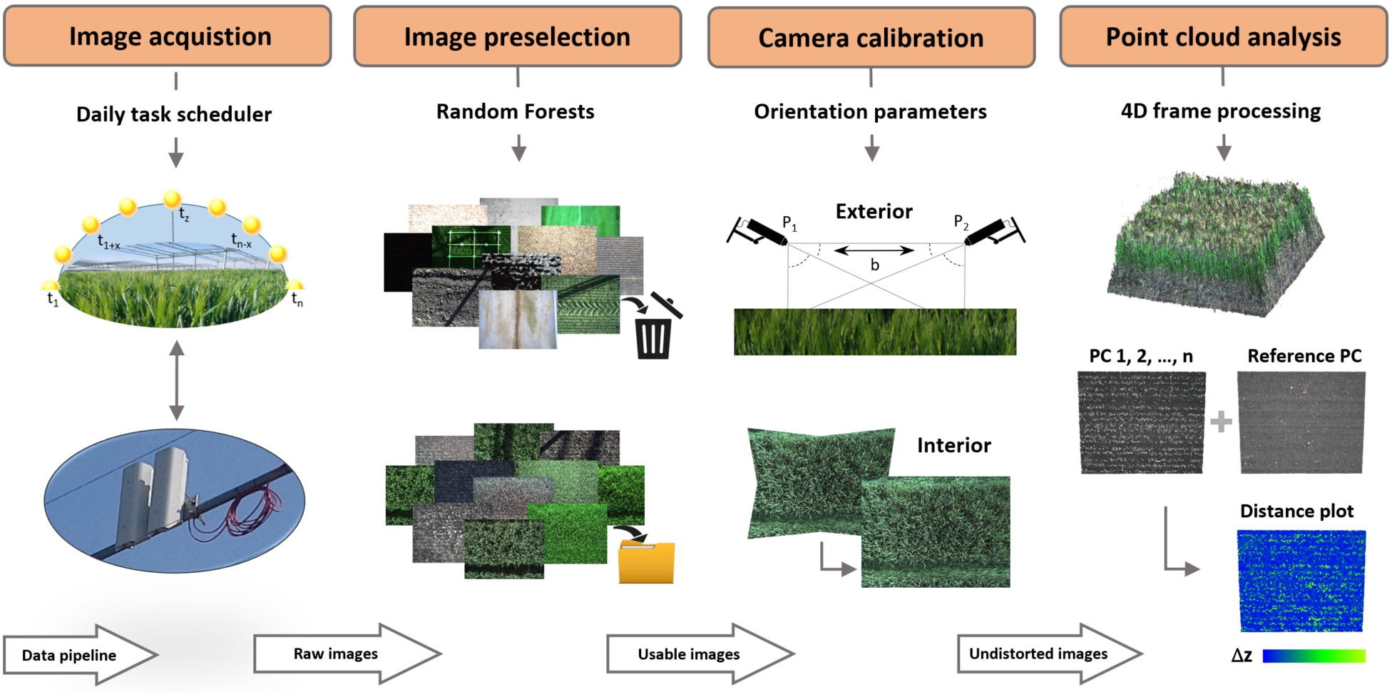
:Precision agriculture relies on understanding crop growth dynamics and plant responses to short-term changes in abiotic factors. In this technical note, we present and discuss a technical approach for cost-effective, non-invasive, time-lapse crop monitoring that automates the process of deriving further plant parameters, such as biomass, from 3D object information obtained via stereo images in the red, green, and blue (RGB) color space. The novelty of our approach lies in the automated workflow, which includes a reliable automated data pipeline for 3D point cloud reconstruction from dynamic scenes of RGB images with high spatio-temporal resolution. The setup is based on a permanent rigid and calibrated stereo camera installation and was tested over an entire growing season of winter barley at the Global Change Experimental Facility (GCEF) in Bad Lauchstädt, Germany. For this study, radiometrically aligned image pairs were captured several times per day from 3 November 2021 to 28 June 2022. We performed image preselection using a random forest (RF) classifier with a prediction accuracy of 94.2% to eliminate unsuitable, e.g., shadowed, images in advance and obtained 3D object information for 86 records of the time series using the 4D processing option of the Agisoft Metashape software package, achieving mean standard deviations (STDs) of 17.3–30.4 mm. Finally, we determined vegetation heights by calculating cloud-to-cloud (C2C) distances between a reference point cloud, computed at the beginning of the time-lapse observation, and the respective point clouds measured in succession with an absolute error of 24.9–35.6 mm in depth direction. The calculated growth rates derived from RGB stereo images match the corresponding reference measurements, demonstrating the adequacy of our method in monitoring geometric plant traits, such as vegetation heights and growth spurts during the stand development using automated workflows.

1. Introduction
The increasing demand for efficient vegetation monitoring and precise determination of crop traits under dynamic environmental conditions has driven remarkable progress in the field of precision agriculture. In particular, remote sensing-based technologies, spatially-explicit data analysis incorporating multiple data sources, and operational workflows have rapidly developed over the past few decades. These advancements have significantly enhanced our understanding and site-specific management of crop growth dynamics, optimization of resource utilization, and the adoption of sustainable agricultural practices. However, continued research and exploration are essential to fully release their potential to deal with processes related to drivers such as climate change [1]. Specifically, the dynamics of grassland and crop systems are complex due to the interaction between biotic (e.g., plant health, species type) and abiotic (e.g., soil moisture, soil temperature) system components, as well as the particular management regime. In this context, a key objective is the comprehensive monitoring of various plant traits including growth, vitality, stress, and biomass volume throughout the principal Biologische Bundesanstalt, Bundessortenamt, and Chemical Industry (BBCH) growth stages of mono- and dicotyledonous plants of an entire growing season [2], which provides information on crop response to changing environmental parameters or extreme climate conditions [3]. In turn, the BBCH classification of phenology plays a key role in the aspired standardization of remote sensing-based vegetation data products as it may link information between different scales of observation (i.e., ground truth vs. satellite scale).
Several cost-effective non-invasive monitoring strategies have been developed that are applicable to research areas encompassing plant phenotyping, agriculture, and crop modeling, e.g., [4,5]. Driven by remote sensing-based monitoring approaches (i.e., Unmanned Aerial Vehicle (UAV), airborne, or satellite), innovative ground truth methods are required that can translate BBCH parameters between scales. For that reason, imaging techniques utilizing digital photogrammetry, in combination with machine vision technologies, are promising as they enable the extraction of plant traits from camera images e.g., [6,7,8]. Numerous recent studies in precision agriculture are dedicated to the campaign-based assessment of geometric plant characteristics, including parameters such as growth height, biomass, leaf morphology, fruit shape, and yield estimation. Those parameters are most effectively captured by techniques that enable the extraction of spatial depth information about an object. Notable examples of such techniques are Light Detection and Ranging (LiDAR), e.g., [9,10], Structure-from-Motion (SfM), which is the three-dimensional reconstruction of structures using a series of two-dimensional RGB images captured from multiple viewpoints, e.g., [11,12,13], the combination of RGB cameras with depth sensors for the simultaneous capturing of color and depth information, e.g., [14,15], or the combination of several of the above-mentioned methods and carrier platforms, e.g., [16,17]. An approach that utilizes two RGB cameras installed in a stereo-capable orientation is referred to as binocular vision or stereoscopic vision, which closely resembles the depth perception of the human eye. Several studies have been conducted using this specific camera configuration, predominantly in field laboratories or pilot-scale experiments, such as isolated chambers or greenhouse tests, e.g., [18,19]. In this context, Dandrifosse et al. [20] discussed the challenges of the laboratory-to-field transition. Some studies that use stereo vision in precision agriculture focus on real-time data analysis, e.g., for camera installations on autonomous harvesters [21,22]. Within all of those applications, the determination of morphological plant features is typically conducted in a campaign-based manner, which is subject to limitations such as dependence on weather conditions and manpower availability. As a result, previously mentioned studies provide discrete snapshots of structural 3D information at specific time points.
To observe plant responses to short-term changes in abiotic factors and to understand the crop growth dynamics under climate change conditions, it is crucial to enhance the spatio-temporal resolution. This can be achieved through continuous monitoring over time and adjustments to the camera-to-object distance, on which the spatial resolution primarily depends [23]. For example, Tanaka et al. [24] attained a ground sampling distance (GSD) of 2 mm per pixel through ground-based image acquisition, while other researchers such as Zhang et al. [25], reported GSD values in the centimeter range per pixel for various flight altitudes of UAV imagery in the context of agricultural monitoring. Several studies have employed stereo vision-based approaches with rigidly installed camera configurations to monitor the morphological and geometric parameters over time [26,27,28,29]. However, current research shows limitations in terms of insufficient spatio-temporal resolution to effectively track dynamic changes in geometric plant traits, such as growth spurts, plant elasticity, or fructification. Additionally, an integrated fully-automated workflow encompassing all stages, ranging from data acquisition to 3D modeling, is missing. Such automated workflows have great potential for future remote sensing-based agricultural products but also for scientific experiments and analysis. With an interface to corresponding management apps, they provide conceivable modules for, e.g., Farm Management Information Systems.
The first objective of this study was to develop a contemporary approach for agricultural vegetation monitoring, such as canopy height and growth rate, by utilizing a permanently installed RGB stereo camera system. The system setup allows for continuous, weather-independent on-site monitoring of crop plants at a high spatio-temporal resolution. Time intervals for the acquisition of image pairs are user-defined, allowing for flexibility in capturing specific time points of interest. The stereo camera system was installed over a test field of winter barley and was tested under controlled conditions during the vegetation period from November 2021 to June 2022. We selected a sampling rate of up to twelve images per day in our study, enabling the precise observation of plant growth dynamics through 3D point cloud reconstruction and facilitating the accurate assessment of morphological plant responses to short-term changes in abiotic parameters. Our second objective was to efficiently and automatically derive primary plant traits from RGB image pairs at any given time. To achieve this, a robust and fully automated data pipeline was developed encompassing image acquisition, classification, and photogrammetric analysis. Additionally, we compared the calculated growth heights and growth rates with regularly conducted reference measurements throughout the main growing season to assess the capabilities and limitations of the system.
2. Experimental Setup
The installation of a high-resolution stereo camera system for 4D vegetation monitoring, i.e., canopy height and biomass response to changes in abiotic factors over time, requires a focus on a setup that ensures the comparability of the cameras in the system, the captured stereo images, and the computed 3D point clouds. To this end, we carefully address the following points in our workflow: (a) System calibration, i.e., respectively, determining the interior orientation and distortion parameters (IOP) and exterior orientation parameters (EOP) of both cameras; (b) Image acquisition, i.e., precise stereo image synchronization and the alignment of stereo image properties (point operations, e.g., histogram alignment) and (c) 3D point cloud generation, i.e., reasonable spatio-temporal resolution in terms of the variation to be expected and measured.
2.1. Field Site: GCEF Bad Lauchstädt
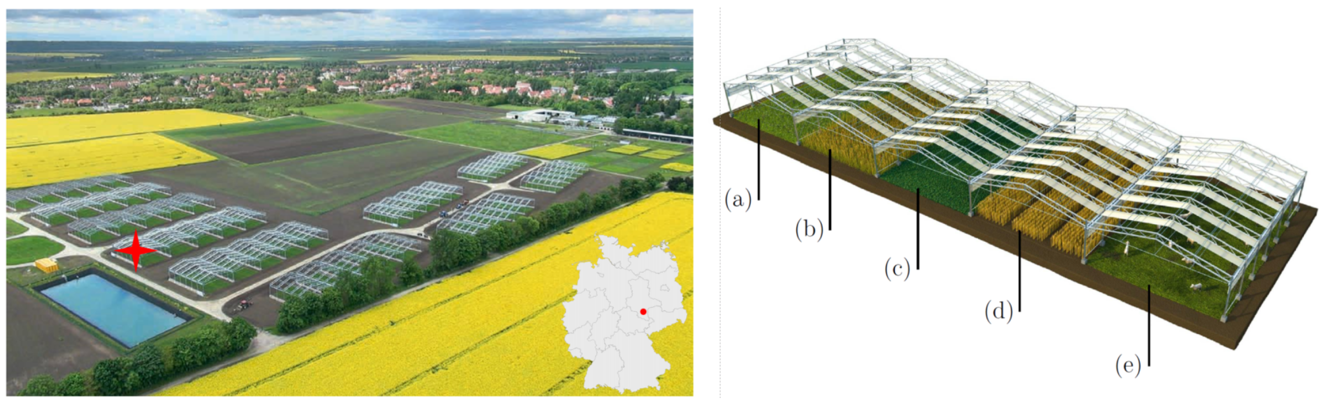
The stereo camera system is installed at the field site of the GCEF located in Bad Lauchstädt, Saxony-Anhalt, Germany (51°23’30”N, 11°52’49”E, see Figure 1). The research facility was designed to investigate the consequences of a future climate scenario for ecosystem functioning in different land-use types of farm- and grassland on several large field plots [30]. Furthermore, GCEF experimental plot data provide an excellent training database for remote sensing-based prediction models. For our study, we have chosen to monitor winter barley that is usually sown in autumn. As an essential cereal in EU agriculture, it is part of the characteristic crop rotation in the present and near-future [31]. Winter barley can develop deeper roots already during the winter months as soil moisture is usually sufficient, which increases its resistance to drought stress in the spring. This and a long growth period make it an ideal observation object to test our stereo setup under different extreme environmental and ambient light conditions.
2.2. Stereo Camera Setup
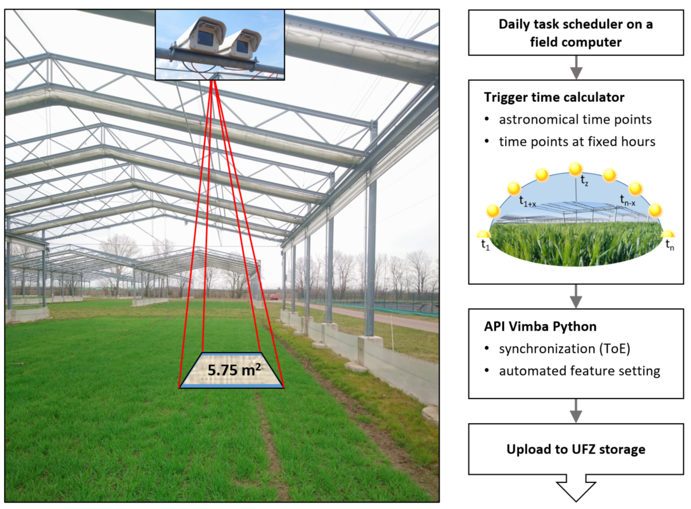
Two parallel arranged RGB frame cameras of the type Mako G-319C (resolution: 2064 × 1544, frames per second: 37.6, pixel size: 3.45 μm; [32]) manufactured by Allied Vision were installed on the roof construction of a GCEF field plot with a camera-to-object distance of about 6.5 m (Figure 2). The cameras are fixed in a stereo-capable orientation with a baseline of about 20 cm in a waterproof hard case with protection standard IP66. Equipped with fixed lenses featuring a 16 mm focal length, they achieve a GSD of 1.45 mm per pixel. In view of the camera-to-object distance and the image overlap of 86.7%, this allows for the three-dimensional observation of a plot size of 2.16 × 2.67 m = 5.75 m2 related to floor level without vegetation. Smaller parts of the crop plants, such as small leaves or ears of corn, can be dissolved in this arrangement. Cameras are controlled by a Pokini i2 field computer (cf. Section 2.3; [33]) and supplied by Power over Ethernet (PoE). To guarantee a stable performance, power outtakes are covered by an uninterruptible power supply (UPS).
2.3. Image Acquisition
Automatic image acquisition, see Figure 2, is part of the automated data pipeline. A key requirement for time-lapse stereo vision is the comparability of the images from the stereo cameras and of the calculated point clouds over time (cf. introduction of Section 2). For this purpose, both cameras were radiometrically adjusted for exposure and white balance using the application programming interface (API) Vimba Python v0.3.1 from Allied Vision Technologies GmbH [34] and synchronously triggered. A multi-threading approach controlled by Trigger over Ethernet (ToE) is used to simultaneously stream several frames per camera into a queue. Meanwhile, bright areas in the frames are detected, and the configuration parameters are iteratively adjusted to ensure that these areas are not saturated once the threshold for the number of frames is reached. Finally, the current frame is saved as an image in the uncompressed Tag Image File Format (TIFF). The image acquisition is controlled by a daily task scheduler. Here, variable astronomical (sunrise, noon, sunset) and constant time intervals of two hours (between 6 am and 10 pm) were chosen to ensure the comparability of point clouds both in high temporal resolution over the entire vegetation period and concerning changes in abiotic parameters.
2.4. Measurement of Reference Data
In order to evaluate the feasibility and quality of the introduced approach, manual canopy height measurements of winter barley were conducted regularly during the main growing season, starting with the principal growth stage 3 of BBCH-scale [2] in mid-April until harvest at the end of June 2022. Plant height is determined by using an ultra-light rectangular polystyrene plate, which is placed on the crop surface at a specified representative location within the overlapping area of stereo image pairs. The height is measured from the ground to the lower edge of the plate on all four sides and then averaged. Thus, the measurement method determines the mean height of a crop surface area and not the maximum height of single plants or awns. In general, canopy height is a reliable estimate of above-ground plant biomass across ecosystems and accordingly, therefore, indicates growth rates [35] and grain yield production [36]. In addition, the current developmental stage of the plants is categorized according to the general stages of the BBCH scale.
3. Data Processing
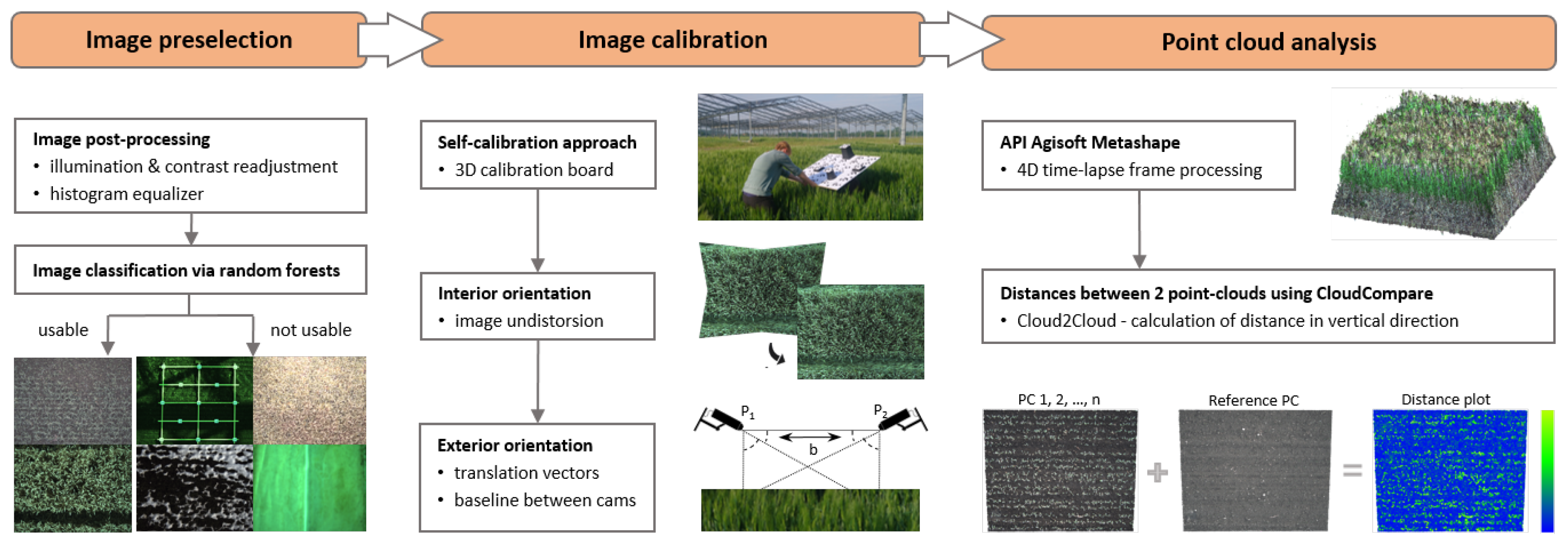
This chapter introduces the part of the data pipeline for generating 3D point clouds from time-lapse stereo images, which includes stereo image preselection, undistortion, and relative orientation, reconstruction of 3D point clouds, and C2C distance calculation to estimate growth heights (Figure 3). The workflow steps are realized using Python.
3.1. Image Preselection
The quality of the 3D reconstruction from time-lapse stereo images is dependent on their image quality (cf. Section 2). Thus, we removed images from the time-lapse series, which were impaired by over- or underexposure, blur, snowfall, snow cover, field operations, or a closed roof covering the field plot (Figure 3). To achieve this, image classification was performed by object recognition with machine learning using Scikit-learn [37]. An RF classifier [38] was chosen to separate the stereo images into two classes: ‘usable’ showing different growth stages of winter barley and ‘not usable’ which are the impaired images. The classifier was trained with 1280 images of the field plot distributed into both classes (usable: 57%, not usable: 43%) and the amount of test data was set to 400 images. Here, the best training parameter set was chosen by using grid search cross-validation over a standard parameter grid. The basis for training variables is formed by histograms of different color bands and color spaces. During classification, i.e., before class prediction, images are temporarily pre-processed by point operations using the libraries of OpenCV [39] and Scikit-image [40]. In detail, we applied histogram matching to all image pairs using a representative reference image and contrast adjustment. If an image is classified as not usable, all images of a certain time stamp are discarded. All usable images are subjected to further processing.
3.2. Camera Calibration
Deriving 3D information, i.e., canopy heights, from stereo images requires knowledge of the stereo geometry of both images, which implies the relative orientation between both images and the IOP of each image. Furthermore, a scale is required to transfer calculated 3D data from a model coordinate system into a metrically-scaled local coordinate system. Both cameras implemented in our stereo camera system use central perspective and could be described by Brown’s standard camera and lens model [41]. The IOP of both cameras was simultaneously determined via camera self-calibration, implemented in AICON 3D Studio v12.00.10 [42]), using a 3D calibration test field that has been captured with synchronized images (see Figure 3; image measurement accuracy, given by , amounted to 0.56 µm). Besides the IOP of both cameras, we received the EOP for each image pair that was used in the calibration process. The pairwise determined EOP, more precisely, the translation vectors, were used to establish the baseline between both cameras, which was used to scale the 3D data in the subsequent processing. In total, translation vectors were available for 86 image pairs, resulting in a mean baseline of 198.41 mm (±11.47 mm).
The images, which have been assessed as suitable in the previous classification for further processing, were undistorted using the determined IOP via an in-house undistortion tool because the software used for relative image orientation and stereo reconstruction does not support the lens distortion model of Brown [41].
3.3. Time-Lapse Stereo Reconstruction
Calculating the relative orientation of each undistorted stereo pair of the time-lapse sequence in a shared model coordinate system was conducted in Agisoft Metashape v1.7.1 using its “Dynamic Scene (4D)” option [43]. In order to scale the 3D data, i.e., to transfer the relatively determined EOP of the stereo images into a metric coordinate system, we used the calculated baseline as a “scale bar” in Metashape (length: 198.41 mm, accuracy: 11 mm). This transforms the EOP of both cameras, which until now have only been available in an arbitrary model coordinate system, into a metric local coordinate system. When using the “Dynamic Scene (4D)” option, the local coordinate system and the EOP are determined only once for the first image pair of the time-lapse stereo sequence and applied to all subsequent stereo images that have been captured, respectively, per time stamp. The stereo camera system is assumed to be statically mounted and rigid with a stable baseline during the entire observation period. The calculation of the camera position and orientation parameters, i.e., the position of the camera’s projection center and the rotation of the camera coordinate system in the object coordinate system, is conducted using the “Align Photos” option that calculates, beside the camera position and orientation parameters, a sparse 3D point cloud from homologous image points via spatial intersection. We performed bundle block adjustment (“Optimize”) to, on the one hand, optimize the determined EOP and on the other hand, to calculate statistics, i.e., the 3D STD for each 3D point of the sparse cloud, whose amount is hereinafter referred to as “precision maps”. Details on those precision estimates are given in James et al. [44,45].
Once the image configuration was established, we used Metashape’s dense image-matching functionality to calculate a dense 3D point cloud for each time stamp. In the following, we used the reconstructed dense clouds together with the precision estimates, calculated for each time stamp and extrapolated to the dense clouds, to derive evidence about the dynamics of plant traits over time. The precision estimates allow for the estimation of the significance of any detected changes with respect to the local accuracies of the computed 3D point clouds.
Finally, to obtain depth information over time, absolute C2C distances were calculated for the entire sequence of reconstructed 3D point clouds related to a reference point cloud, in our case the date of the first plant emergence on 3 November 2021. For distance determination, the nearest neighbor distance based on a kind of Hausdorff distance algorithm, was used that is implemented in the open source software CloudCompare v.2.13 [46,47]. Furthermore, it should be noted that the error calculation performed in addition to the C2C distances calculation is based on Gaussian error propagation.
4. Results
The stereo camera system has reliably captured RGB images of a winter barley field several times a day from 3 November 2021, to 28 June 2022, and provided the database to quantify the canopy height of the winter barley test plots. In total eight to twelve stereo image pairs were captured per day, 4790 images in sum. To investigate the setup capabilities over the whole growth period we have analyzed one image pair per three days in the winter time and one image pair per two days from the end of March 2022 resulting in 86 image pairs. To ensure comparability due to ambient light conditions, we have chosen to analyze the first image pair of each day.
4.1. Image Classification Using Machine Learning
The classification of 400 test images into the two classes ‘usable’ and ‘not usable’ resulted in an accuracy score of 0.9575 for the optimal parameter configuration. The resulting 2 × 2 error matrix A provides insights into prediction outcomes. In the ‘usable’ class, which encompasses 229 images, A1 = [226,3] denotes the accurate classification of 226 usable pictures and three misclassifications. For the ‘not-usable’ class, comprising 171 images, A2 = [14,157] reveals 14 misclassifications and the correct classification of 157 images. The class report for ‘usable’ shows a precision of 0.94 and a recall of 0.99. The ‘not-usable’ class yielded a precision of 0.98 and a recall of 0.92, both determined from the test run. However, during the preselection of the plot image data, about 94.2% (89.6–99.8% per month) of all captured images were correctly classified. Images with impaired effects, cf. Section 3.1, were reliably removed with a prediction accuracy of 94.1%. On the other hand, several potentially usable images were falsely classified as not usable, 5.7% in sum and were, therefore, not considered further. These results fit a mean accuracy score for the classifiers’ prediction of test data of 0.9425 ± 0.0275 obtained from k-fold cross-validation with 10 folds.
4.2. 3D Point Clouds: Reconstruction, Evaluation, Distances
The 3D stereo reconstruction of 86 sparse clouds was conducted within a precision of 11.4–80.6 mm in the depth direction, which, in mathematical notation, represents and is stored in precision maps (cp. Section 3.3). The calculation of the 98th percentile cut very few outliers and reduced this range to an interval of 23.1–64.5 mm. Arithmetic means of the STDs values were found to be in the range of 17.3–30.4 mm. The medians of the STDs values fell within the range of 16.9–26.9 mm.
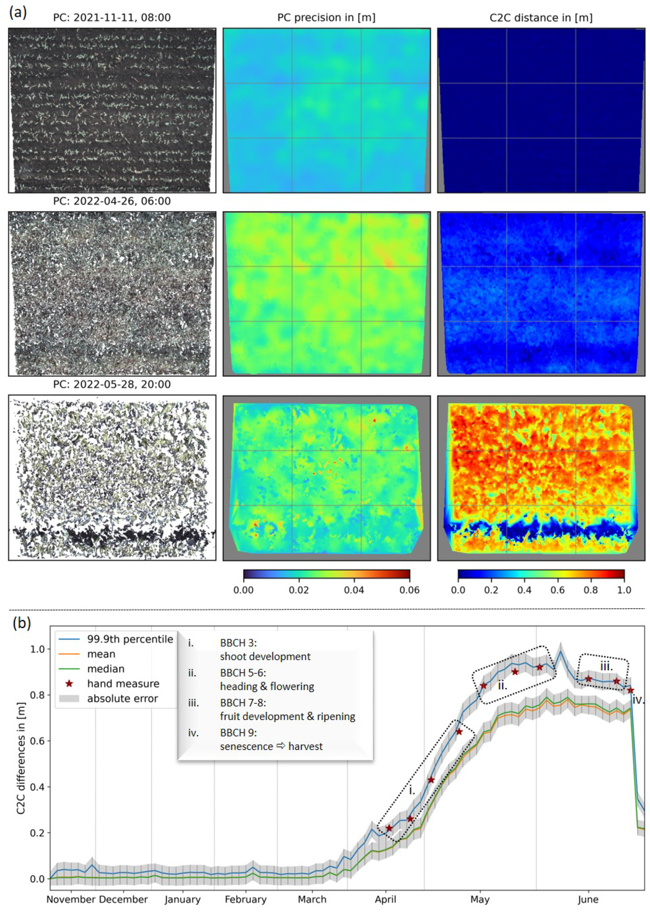
Figure 4a displays exemplary results of the 3D stereo reconstruction, the accompanied interpolated precision maps, and the C2C distance calculation at three points in time of our measurement series. Since the stereo camera system is mounted at a slight angle to the perpendicular, the graphics show a trapezoidal shape from the top to the bottom of a single image, whose extent decreases with plant growth over time due to the fixed field of view of our stereo cameras. Additionally, we observed a decrease in point cloud density with increasing crop growth (Figure 4a; 1st column). At the same time, the point cloud precision decreased with the point cloud density (Figure 4a; second column). This effect can also be observed in Table 1(b). The intervals for STDs reveal a trend indicating an anti-correlation between the point cloud density and the maximum STD values. For example, we observed the range of STDs in the depth direction and the accompanied anti-correlated point cloud density to be 16.7–24.8 mm/5.3 M points, 19.0–40.8 mm/4.2 M points and 12.7–54.8 mm/2.9 M points with the increasing time steps in Figure 4a (see also Table 1; dates are marked with *). For these dates, the calculation of the 98th percentile reveals maximum values of 22.6 mm, 34.0 mm, 33.8 mm, respectively, and therefore, cuts the few outliers shown as dark-red dots in the precision maps. The mean/median STDs range from 19.6 mm/19.4 mm to 28.9 mm/28.8 mm. C2C distances were calculated concerning the reference date, 3 November 2021. The results map the crop surface (Figure 4a; 3rd column) and, thus, represent the current maximum vegetation height. For visualization, gaps within the calculated C2C distance maps were interpolated. At later observation times, for example, on 28 May 2022, significant height variations become evident. The distinct blue line, indicating near-zero heights, can be correlated with the track of a fertilizer vehicle (as also visible in Figure 2).
Due to interpolation artifacts at the edges of the plots resulting from the C2C distance calculation steps and human-made impacts, such as vehicle tracks or footpaths, further analysis was limited to an undisturbed area, specifically the central cell of the 3 × 3 grid drawn on the images in Figure 4a. Based on this, a seasonal time-series of distance calculations is displayed in Figure 4b, and furthermore, related values for representative dates are written in Table 1(a). The resulting curves exhibit similar slopes and are enclosed by a gray ribbon representing the absolute error calculated using Gaussian error propagation. The curves of the mean (orange) and median (green) height values are almost congruent and only start to diverge with increasing plant height, which is also evident from Table 1(a). A comparison of average values for maximum growth heights (blue curve) with manual height measurements (red stars) is conducted by calculation of a 99.9th percentile for the observed rectangle. These average values take into account the temporal flattening of the surface due to the hand measurement method used (cf. Section 2.4). Both the determination of maximum height and growth dynamics according to principal BBCH stages are consistent for hand and camera measurements within error intervals (Table 1(a)). The absolute error is slightly correlated with vegetation height and ranges between 24.9 mm and 35.6 mm over the entire time series. Finally, all of the displayed curves collapsed to the swath height on 28 June 2022, due to the harvest of the field plot on this date. The observations and hypotheses described in this section are supported by the values in the last two rows of Table 1, i.e., median/mean converge, error values drop, and point cloud density increases with an abrupt decrease in vegetation height.
5. Discussion
The approach presented combines continuous vegetation monitoring using stereo-vision photogrammetry for high spatio-temporal vegetation parameter monitoring. The experiment shows proof of principle for the retrieval of canopy height within an autonomous ground truth solution. The presented automated data pipeline includes the acquisition, classification, and photogrammetric analysis of RGB image data, and thus, the automatic derivation of geometric plant traits from the 3D reconstruction of stereo image pairs. As demonstrated in this study, the sampling rate of about eight to twelve image pairs per day over a whole growing season enables the possibility to reliably and closely determine heights or growth rates, which allows for the investigation of plant response to short-term changes in abiotic environmental conditions related to plant geometry and growth.
However, long-term observation in a non-laboratory environment is a technical challenge [28], especially for a permanently installed system. A range of factors can interfere with data acquisition and affect the quality of stereo image pairs or, in the worst case, interrupt the monitoring. First, power outages due to, e.g., construction work at the field site or unexpected problems in the electricity supply caused recurring gaps in our time-series and later resulted in the installation of a UPS. Second, the quality of captured images can be affected by varying ambient light conditions during the camera configuration (cf. Section 2.3). Fast light–shadow changes due to clouds, sunlight reflection on the leaves, and also minor snow patches can lead to the wrong adjustment of white balance and exposure, resulting in overexposed images. Third, we also captured images showing snow cover or a closed construction roof. Thus, the pre-classification of image pairs was required before applying further 4D processing steps.
In this study, we used a simple supervised RF classifier to remove unsuitable stereo-image pairs from the data pipeline. The selection of 4790 stereo images into usable or not usable data using histograms succeeded in a satisfactory 94.2%. According to Millard and Richardson [48] RF is generally appropriate for RGB image classification, but better results could be achieved by adjusting the amount and selection of training data as well as strictly equalizing the training images within the number of groups. Additionally, a comprehensive test using cross-validation and grid search across a range of specific input variables can enhance accuracy by identifying the optimal variable combination for training the model. The application of further classifiers could also increase the prediction accuracy [49]. Note, for more complex classification approaches in precision agriculture, e.g., phenotyping, detecting plant diseases, observing BBCH stages, counting fruit bodies, or similar classifiers, e.g., [50,51] or a deep learning approach [52] could be more appropriate. Certainly, with regard to the extent of the applicability to various plant types and observation sites, the exploration of unsupervised learning algorithms becomes particularly relevant. In cases of generating new training datasets for distinct vegetation types with annotations, unsupervised image classifiers demonstrate clear advantages over their supervised counterparts in terms of data curation effort and processing time.
The 3D point cloud reconstruction provides reliable results. The theoretically achievable object point accuracy can be estimated separately for position and depth by applying the error propagation law when assuming the stereo normal case (details are given in [53], p. 35), which amounts to 1 mm and 23 mm concerning our setup. Note, that theoretical accuracy is a limiting factor for the observation of geometric parameters, and therefore, must be included in the considerations of an appropriate setup. In our study, the determined STDs of the reconstructed 3D points range in the same order of magnitude (Metashape: 11.4–80.6 mm; 98th percentile: 11.4–64.5 mm), as is the range of the STDs mean and median values of 17.3–30.4 mm and 16.9–26.9 mm, respectively, and the range of the absolute error of 24.9–35.6 mm obtained by C2C calculation. Image measurement and matching of homologous points in the stereo image pair are significant factors impacting the accuracy of the object points to be reconstructed. With increasing vegetation height, the detection of homologous points becomes more and more difficult due to varying perspectives and the probability of mismatches increases, e.g., both images capture different sides of upright leaves, awns, and fruits. Any gaps in the point clouds are due to superimposed vegetation causing mutual occlusions (Figure 4a). Furthermore, Table 1(b) demonstrates a clear trend of an inverse relationship between point cloud density and the STDs achieved. This is primarily a result of the increased presence of outliers, which have a more pronounced impact on the mean than on the median, leading to an increasing divergence between the mean and median height curves (cp. Figure 4b and Table 1(a)). Any discontinuities in the marginal areas of the plots shown in Figure 4a result from interpolation errors due to a greatly reduced point density in the marginal area covered by high vegetation. Consequently, the elevation values presented at the margins of the observed study area should be viewed with caution. Anyway, the accuracy of 3D point cloud reconstruction as well as the point cloud density can be increased by using additional cameras within the setup, as stereo image matching would detect more homologous points due to a higher number of ray intersections, e.g., to better deal with occlusions. However, a reasonable cost-benefit calculation in terms of, e.g., the number of cameras, available mounting stations, etc., is necessary for a field application of our approach on a farm.
A critical aspect of our approach is the geometric stability of the camera setup. Currently, we assume that both the IOP and EOP of both cameras remain stable over the entire observation period. The camera setup was designed for outdoor use, installed in robust, waterproof housings, and firmly mounted to the steel structure above the plot. Elias et al. [54], however, demonstrated that based on low-cost cameras the accumulation of waste heat, which is to be expected as a result of the housing construction, likely has an impact on the physical integrity of the camera. Furthermore, they show that the temporal stability of the calibration parameters is influenced by environmental factors, e.g., sunlight and cold. In particular, changes in the principal point and principal distance are to be expected, which in turn, are directly correlated with the depth measurement. Consequently, it is recommended that the calibration, i.e., the IOP, of both cameras is inspected regularly and updated if required. The same applies to the EOP of both cameras, respectively, and their relative orientation. Even if the installation is most stable, weather impacts on the temporal stability of the position and orientation of the involved cameras cannot be excluded. Accordingly, the EOP should likewise regularly be verified and, if necessary, updated. For both, on-the-job calibration using a sufficient number of ground control points in the field of view should be considered.
The data pipeline for plant monitoring with a stereo camera system can be improved concerning the aspects previously discussed. Transferability to other practical agricultural applications is conceivable since the pipeline is automated, starting with the high-resolution data acquisition. As the data analysis consists of modules, it can be supplemented by further methods of photogrammetric data analysis or computer vision. In summary, this is a promising application for service companies in precision farming and a promising tool for fundamental research on vegetation dynamics under global change.
6. Conclusions and Outlook
We presented a robust, cost-effective, non-invasive system for potential long-term crop monitoring and associated automated analysis of geometric plant traits for precise agricultural applications, such as biomass, canopy height, or Leaf Area Index (LAI). The high spatio-temporal resolution allows for the correlation of stereo vision-based 3D depth information to abiotic parameters in terms of, e.g., growth spurts, plant elasticity, or fructification. A unique feature compared to the current use of drones is the potential of weather-independent continuous monitoring with a suitable, automated, and expendable processing pipeline. In principle, the workflow is transferable to drone applications in precision agriculture.
One point to note about the overall workflow package, however, is that the camera calibration procedure is not fully automated, i.e., it is advisable to calibrate the system regularly to control the stability of the IOP. A critical point of the data pipeline concerns the compilation of an appropriate RF training data set for each specific installation site. In this state, an agronomic service is still required.
Considering the workflow as a sequential arrangement, it is conceivable to augment the data analysis with supplementary methodologies, such as detecting geometrical objects using machine learning, once the 3D point clouds have been reconstructed. Perpendicular porosity of the vertical foliage walls, plant geometry under changing sunlight or wind conditions, or observation of BBCH stages correlated to climatic events are influencing environmental effects, which should be the subject of future observations in order to improve the workflows’ validity of results. For example, our study will be extended to another non-greenhouse field plot at the GCEF for evaluation reasons and to examine crop growth with respect to abiotic parameters by comparing a manipulated and a non-manipulated plot. Furthermore, the implementation of the presented or similar workflows may be conducted by using sophisticated open-source software like COLMAP v3.9.1 [55] in the future.
Further potential for use cases in agriculture lies in the processing of the color information of the recorded images. These data can be used to determine the optimal timing for the harvest of crops from images, e.g., utilizing machine learning for detecting flowering [56]. In situ stereo-vision camera data may provide ground truth information for UAV or satellite-based color mapping for this purpose. Additionally, the detection of diseases, deficiencies, and stress symptoms in plants is enabled by the color information. This can be conducted, among other things, using spectral vegetation indices. In the setup described here with RGB images, e.g., the application of the Visible Atmospherically Resistant Index may be appropriate, which is designed to estimate vegetation fraction in the visible portion of the spectrum [57]. Using color information to differentiate between weeds and crops enables the precise application of herbicides for weed control while at the same time protecting the crops. Therefore, several weed detection methods based on computer vision [58] involve color information to improve crop productivity. Furthermore, stereo vision-based geometric plant data could be extended by further remote sensing-based observations, e.g., of the near-infrared (NIR), short-wave infrared (SWIR), and thermal infrared (TIR) spectral bands. Especially, the combined analysis of plant geometric data and thermal emissivity may support research and parameter retrieval for evapotranspiration and plant health scenarios under changing environmental conditions [59,60].
In conclusion, there is potential for further investigation regarding the camera setup and the data pipeline. Higher accuracy and density of the reconstructed 3D point clouds could be achieved by using multi-image techniques, as a larger number of cameras can capture the object with multiple convergent images to reduce stereo reconstruction ambiguities and occlusions, e.g., [61]. Here, RGB and thermal oblique camera solutions [62] provide innovative observations and may be coupled to the 3D point cloud reconstruction. Experiments using UAV-based data acquisition at various spatial scales also provide a cost-efficient method to study scaling effects in point cloud reconstruction quality. However, one significant added value of the described actual setup lies in the utilization of established, passive, non-invasive measurement techniques, resulting in minimal costs and substantial gains, even if it entails accepting certain trade-offs, e.g., decreasing accuracy measures or point cloud density with increasing plant height. Building upon the presented data pipeline and included processes, the potential for enhancing output quality and expanding applicability to diverse vegetation types and observation sites is evident through the incorporation of additional methods in data curation, analysis, and error estimation.
Author Contributions
Conceptualization, J.B. and H.M.; methodology, J.B. and H.M.; setup, H.M. and M.K.; data pipeline & software & validation, M.K. and M.E.; reference measurement, I.M.; site management, M.S.; writing—original draft preparation, M.K., M.E., H.M. and M.P.; visualization, M.K.; supervision, H.M.; project administration, H.M.; funding acquisition, H.M. All authors have read and agreed to the published version of the manuscript.
Funding
This research was funded by the Federal Ministry of Food and Agriculture, grant number 28DE102B18.
Data Availability Statement
The data presented in this study are available upon request from the corresponding author. The data are not publicly available due to personal data protection laws for imaging data.
Acknowledgments
This study is part of the EXPRESS project which addresses the above key issues and supports farmers with the development of modern monitoring strategies in the selection of suitable crops, their cultivation and maintenance. The GCEF is funded by the Federal Ministry of Education and Research, the State Ministry for Science and Economy of Saxony-Anhalt and the State Ministry for Higher Education, Research, and the Arts of Saxony. Additional thanks to Konrad Kirsch and Ines Merbach for their excellent fieldwork and support. Furthermore, we gratefully thank Frank Liebold for providing a tool for image undistortion using Brown’s camera and lens model.
Conflicts of Interest
The authors declare that they have no known competing financial interests or personal relationships that could have appeared to influence the work reported in this paper.
References
- Mulla, D.J. Twenty five years of remote sensing in precision agriculture: Key advances and remaining knowledge gaps. Biosyst. Eng. 2013, 114, 358–371. [Google Scholar] [CrossRef]
- Meier, U. Growth Stages of Mono- and Dicotyledonous Plants: BBCH Monograph; Open Agrar Repositorium: Quedlinburg, Germany, 2018; p. 204. [Google Scholar] [CrossRef]
- Morison, J.I.; Morecroft, M.D. Plant Growth and Climate Change; John Wiley & Sons: Hoboken, NJ, USA, 2008. [Google Scholar]
- Vázquez-Arellano, M.; Griepentrog, H.W.; Reiser, D.; Paraforos, D.S. 3-D imaging systems for agricultural applications-—A review. Sensors 2016, 16, 618. [Google Scholar] [CrossRef]
- Li, L.; Zhang, Q.; Huang, D. A review of imaging techniques for plant phenotyping. Sensors 2014, 14, 20078–20111. [Google Scholar] [CrossRef] [PubMed]
- Wakchaure, M.; Patle, B.; Mahindrakar, A. Application of AI Techniques and Robotics in Agriculture: A Review. Artif. Intell. Life Sci. 2023, 3, 100057. [Google Scholar] [CrossRef]
- Kolhar, S.; Jagtap, J. Plant trait estimation and classification studies in plant phenotyping using machine vision–A review. Inf. Process. Agric. 2021, 10, 114–135. [Google Scholar] [CrossRef]
- Li, Z.; Guo, R.; Li, M.; Chen, Y.; Li, G. A review of computer vision technologies for plant phenotyping. Comput. Electron. Agric. 2020, 176, 105672. [Google Scholar] [CrossRef]
- Blanquart, J.E.; Sirignano, E.; Lenaerts, B.; Saeys, W. Online crop height and density estimation in grain fields using LiDAR. Biosyst. Eng. 2020, 198, 1–14. [Google Scholar] [CrossRef]
- Schirrmann, M.; Hamdorf, A.; Garz, A.; Ustyuzhanin, A.; Dammer, K.H. Estimating wheat biomass by combining image clustering with crop height. Comput. Electron. Agric. 2016, 121, 374–384. [Google Scholar] [CrossRef]
- Ji, Y.; Chen, Z.; Cheng, Q.; Liu, R.; Li, M.; Yan, X.; Li, G.; Wang, D.; Fu, L.; Ma, Y.; et al. Estimation of plant height and yield based on UAV imagery in faba bean (Vicia faba L.). Plant Methods 2022, 18, 1–13. [Google Scholar] [CrossRef]
- Volpato, L.; Pinto, F.; González-Pérez, L.; Thompson, I.G.; Borém, A.; Reynolds, M.; Gérard, B.; Molero, G.; Rodrigues, F.A., Jr. High throughput field phenotyping for plant height using UAV-based RGB imagery in wheat breeding lines: Feasibility and validation. Front. Plant Sci. 2021, 12, 591587. [Google Scholar] [CrossRef]
- Kröhnert, M.; Anderson, R.; Bumberger, J.; Dietrich, P.; Harpole, W.S.; Maas, H.G. Watching grass grow-a pilot study on the suitability of photogrammetric techniques for quantifying change in aboveground biomass in grassland experiments. ISPRS Int. Arch. Photogramm. Remote Sens. Spat. Inf. Sci 2018, 42, 539–542. [Google Scholar] [CrossRef]
- Rueda-Ayala, V.P.; Peña, J.M.; Höglind, M.; Bengochea-Guevara, J.M.; Andújar, D. Comparing UAV-based technologies and RGB-D reconstruction methods for plant height and biomass monitoring on grass ley. Sensors 2019, 19, 535. [Google Scholar] [CrossRef] [PubMed]
- Vit, A.; Shani, G. Comparing RGB-D sensors for close range outdoor agricultural phenotyping. Sensors 2018, 18, 4413. [Google Scholar] [CrossRef]
- Jimenez-Berni, J.A.; Deery, D.M.; Rozas-Larraondo, P.; Condon, A.T.G.; Rebetzke, G.J.; James, R.A.; Bovill, W.D.; Furbank, R.T.; Sirault, X.R. High throughput determination of plant height, ground cover, and above-ground biomass in wheat with LiDAR. Front. Plant Sci. 2018, 9, 237. [Google Scholar] [CrossRef]
- Wang, X.; Singh, D.; Marla, S.; Morris, G.; Poland, J. Field-based high-throughput phenotyping of plant height in sorghum using different sensing technologies. Plant Methods 2018, 14, 1–16. [Google Scholar] [CrossRef]
- Bernotas, G.; Scorza, L.C.; Hansen, M.F.; Hales, I.J.; Halliday, K.J.; Smith, L.N.; Smith, M.L.; McCormick, A.J. A photometric stereo-based 3D imaging system using computer vision and deep learning for tracking plant growth. GigaScience 2019, 8, giz056. [Google Scholar] [CrossRef]
- Tilneac, M.; Dolga, V.; Grigorescu, S.; Bitea, M. 3D stereo vision measurements for weed-crop discrimination. Elektron. Elektrotechnika 2012, 123, 9–12. [Google Scholar] [CrossRef]
- Dandrifosse, S.; Bouvry, A.; Leemans, V.; Dumont, B.; Mercatoris, B. Imaging wheat canopy through stereo vision: Overcoming the challenges of the laboratory to field transition for morphological features extraction. Front. Plant Sci. 2020, 11, 96. [Google Scholar] [CrossRef]
- Wen, J.; Yin, Y.; Zhang, Y.; Pan, Z.; Fan, Y. Detection of Wheat Lodging by Binocular Cameras during Harvesting Operation. Agriculture 2022, 13, 120. [Google Scholar] [CrossRef]
- Bao, Y.; Tang, L. Field-based robotic phenotyping for sorghum biomass yield component traits characterization using stereo vision. IFAC-PapersOnLine 2016, 49, 265–270. [Google Scholar] [CrossRef]
- Eltner, A.; Hoffmeister, D.; Kaiser, A.; Karrasch, P.; Klingbeil, L.; Stöcker, C.; Rovere, A. UAVs for the Environmental Sciences: Methods and Applications; WBG Academic in Wissenschaftliche Buchgesellschaft (WBG): Darmstadt, Germany, 2022; Chapter 1.5.1.2. [Google Scholar]
- Tanaka, Y.; Watanabe, T.; Katsura, K.; Tsujimoto, Y.; Takai, T.; Tanaka, T.S.T.; Kawamura, K.; Saito, H.; Homma, K.; Mairoua, S.G.; et al. Deep learning enables instant and versatile estimation of rice yield using ground-based RGB images. Plant Phenomics 2023, 5, 0073. [Google Scholar] [CrossRef]
- Zhang, J.; Wang, C.; Yang, C.; Xie, T.; Jiang, Z.; Hu, T.; Luo, Z.; Zhou, G.; Xie, J. Assessing the effect of real spatial resolution of in situ UAV multispectral images on seedling rapeseed growth monitoring. Remote Sens. 2020, 12, 1207. [Google Scholar] [CrossRef]
- Zaji, A.; Liu, Z.; Xiao, G.; Bhowmik, P.; Sangha, J.S.; Ruan, Y. Wheat Spikes Height Estimation Using Stereo Cameras. IEEE Trans. Agrifood Electron. 2023, 1, 15–28. [Google Scholar] [CrossRef]
- Cai, J.; Kumar, P.; Chopin, J.; Miklavcic, S.J. Land-based crop phenotyping by image analysis: Accurate estimation of canopy height distributions using stereo images. PLoS ONE 2018, 13, e0196671. [Google Scholar] [CrossRef]
- Brocks, S.; Bareth, G. Estimating barley biomass with crop surface models from oblique RGB imagery. Remote Sens. 2018, 10, 268. [Google Scholar] [CrossRef]
- Schima, R.; Mollenhauer, H.; Grenzdörffer, G.; Merbach, I.; Lausch, A.; Dietrich, P.; Bumberger, J. Imagine all the plants: Evaluation of a light-field camera for on-site crop growth monitoring. Remote Sens. 2016, 8, 823. [Google Scholar] [CrossRef]
- Schädler, M.; Buscot, F.; Klotz, S.; Reitz, T.; Durka, W.; Bumberger, J.; Merbach, I.; Michalski, S.G.; Kirsch, K.; Remmler, P.; et al. Investigating the consequences of climate change under different land-use regimes: A novel experimental infrastructure. Ecosphere 2019, 10, e02635. [Google Scholar] [CrossRef]
- Ballot, R.; Guilpart, N.; Jeuffroy, M.-H. The first map of crop sequence types in Europe over 2012–2018. Earth Syst. Sci. Data 2023, 15, 5651–5666. [Google Scholar] [CrossRef]
- Allied Vision Technologies GmbH. Mako Technical Manual. 2023. Available online: https://cdn.alliedvision.com/fileadmin/content/documents/products/cameras/Mako/techman/Mako_TechMan_en.pdf (accessed on 18 January 2024).
- EXTRA Computer GmbH. Pokini i2 Data Sheet. 2023. Available online: https://os.extracomputer.de/b10256/devpokini/wp-content/uploads/2020/07/Pokini-I2_Datenblatt_DE_V1-2_02-2020_web.pdf (accessed on 18 January 2024).
- Allied Vision Technologies GmbH. About. 2023. Available online: https://www.alliedvision.com/ (accessed on 18 January 2024).
- Proulx, R. On the general relationship between plant height and aboveground biomass of vegetation stands in contrasted ecosystems. PLoS ONE 2021, 16, e0252080. [Google Scholar] [CrossRef] [PubMed]
- Walter, J.D.; Edwards, J.; McDonald, G.; Kuchel, H. Estimating biomass and canopy height with LiDAR for field crop breeding. Front. Plant Sci. 2019, 10, 1145. [Google Scholar] [CrossRef]
- Van der Walt, S.; Schönberger, J.L.; Nunez-Iglesias, J.; Boulogne, F.; Warner, J.D.; Yager, N.; Gouillart, E.; Yu, T. scikit-image: Image processing in Python. PeerJ 2014, 2, e453. [Google Scholar] [CrossRef]
- Breiman, L. Random forests. Mach. Learn. 2001, 45, 5–32. [Google Scholar] [CrossRef]
- Bradski, G. The openCV library. Dr. Dobb’s J. Softw. Tools Prof. Program. 2000, 25, 120–123. [Google Scholar]
- Pedregosa, F.; Varoquaux, G.; Gramfort, A.; Michel, V.; Thirion, B.; Grisel, O.; Blondel, M.; Prettenhofer, P.; Weiss, R.; Dubourg, V.; et al. Scikit-learn: Machine learning in Python. J. Mach. Learn. 2011, 12, 2825–2830. [Google Scholar]
- Brown, D.C. Close-range camera calibration. Photogramm. Eng 1971, 37, 855–866. [Google Scholar]
- Godding, R. Camera Calibration. In Handbook of Machine and Computer Vision; John Wiley & Sons, Ltd.: Hoboken, NJ, USA, 2017. [Google Scholar] [CrossRef]
- Agisoft Helpdesk Portal. 4D Processing. 2022. Available online: https://agisoft.freshdesk.com/support/solutions/articles/31000155179-4d-processing (accessed on 18 January 2024).
- James, M.R.; Antoniazza, G.; Robson, S.; Lane, S.N. Mitigating systematic error in topographic models for geomorphic change detection: Accuracy, precision and considerations beyond off-nadir imagery. Earth Surf. Process. Landf. 2020, 45, 2251–2271. [Google Scholar] [CrossRef]
- James, M.R.; Robson, S.; Smith, M.W. 3-D uncertainty-based topographic change detection with structure-from-motion photogrammetry: Precision maps for ground control and directly georeferenced surveys. Earth Surf. Process. Landf. 2017, 42, 1769–1788. [Google Scholar] [CrossRef]
- Girardeau-Montaut, D. CloudCompare. Fr. EDF R&D Telecom ParisTech 2016, 11, 5. [Google Scholar]
- Huttenlocher, D.P.; Klanderman, G.A.; Rucklidge, W.J. Comparing images using the Hausdorff distance. IEEE Trans. Pattern Anal. Mach. Intell. 1993, 15, 850–863. [Google Scholar] [CrossRef]
- Millard, K.; Richardson, M. On the importance of training data sample selection in random forest image classification: A case study in peatland ecosystem mapping. Remote Sens. 2015, 7, 8489–8515. [Google Scholar] [CrossRef]
- Sheykhmousa, M.; Mahdianpari, M.; Ghanbari, H.; Mohammadimanesh, F.; Ghamisi, P.; Homayouni, S. Support Vector Machine Versus Random Forest for Remote Sensing Image Classification: A Meta-Analysis and Systematic Review. IEEE J. Sel. Top. Appl. Earth Obs. Remote Sens. 2020, 13, 6308–6325. [Google Scholar] [CrossRef]
- Peña, J.M.; Gutiérrez, P.A.; Hervás-Martínez, C.; Six, J.; Plant, R.E.; López-Granados, F. Object-based image classification of summer crops with machine learning methods. Remote Sens. 2014, 6, 5019–5041. [Google Scholar] [CrossRef]
- Kumar, S.; Kaur, R. Plant disease detection using image processing—A review. Int. J. Comput. Appl. 2015, 124. [Google Scholar] [CrossRef]
- Zhou, C.L.; Ge, L.M.; Guo, Y.B.; Zhou, D.M.; Cun, Y.P. A comprehensive comparison on current deep learning approaches for plant image classification. In Proceedings of the Journal of Physics: Conference Series; IOP Publishing: Bristol, UK, 2021; Volume 1873, p. 012002. [Google Scholar] [CrossRef]
- Kraus, K. Photogrammetry, 2nd ed.; DE GRUYTER: Berlin, Germany, 2007. [Google Scholar] [CrossRef]
- Elias, M.; Eltner, A.; Liebold, F.; Maas, H.G. Assessing the Influence of Temperature Changes on the Geometric Stability of Smartphone- and Raspberry Pi Cameras. Sensors 2020, 20, 643. [Google Scholar] [CrossRef] [PubMed]
- Schoenberger, J.L. COLMAP. 2023. Available online: https://colmap.github.io/index.html (accessed on 18 January 2024).
- Kim, T.K.; Kim, S.; Won, M.; Lim, J.H.; Yoon, S.; Jang, K.; Lee, K.H.; Park, Y.D.; Kim, H.S. Utilizing machine learning for detecting flowering in mid-range digital repeat photography. Ecol. Model. 2021, 440, 109419. [Google Scholar] [CrossRef]
- Gitelson, A.A.; Kaufman, Y.J.; Stark, R.; Rundquist, D. Novel algorithms for remote estimation of vegetation fraction. Remote Sens. Environ. 2002, 80, 76–87. [Google Scholar] [CrossRef]
- Wu, Z.; Chen, Y.; Zhao, B.; Kang, X.; Ding, Y. Review of weed detection methods based on computer vision. Sensors 2021, 21, 3647. [Google Scholar] [CrossRef] [PubMed]
- Gerhards, M.; Rock, G.; Schlerf, M.; Udelhoven, T. Water stress detection in potato plants using leaf temperature, emissivity, and reflectance. Int. J. Appl. Earth Obs. Geoinf. 2016, 53, 27–39. [Google Scholar] [CrossRef]
- Sobrino, J.A.; Del Frate, F.; Drusch, M.; Jiménez-Muñoz, J.C.; Manunta, P.; Regan, A. Review of thermal infrared applications and requirements for future high-resolution sensors. IEEE Trans. Geosci. Remote Sens. 2016, 54, 2963–2972. [Google Scholar] [CrossRef]
- Maas, H.G. Mehrbildtechniken in der Digitalen Photogrammetrie. Habilitation Thesis, ETH Zurich, Zürich, Switzerland, 1997. [Google Scholar] [CrossRef]
- Lin, D.; Bannehr, L.; Ulrich, C.; Maas, H.G. Evaluating thermal attribute mapping strategies for oblique airborne photogrammetric system AOS-Tx8. Remote Sens. 2019, 12, 112. [Google Scholar] [CrossRef]
Figure 1.
Overview of the field site and the crop cultivation. (Left): GCEF, its location in Germany, and the location of the camera setup on one of the experimental plots (red star). (Right): Scheme of simulated land-use forms at the facility-a: extensive grassland use (mowing), b: ecological agriculture, c: intensive grassland use, d: conventional production and e: extensive grassland use (grazing) (Illustration: Tricklabor, Marc Hermann, copyright by UFZ, 2014).

Figure 2.
Left: Stereo camera system observing the corresponding vegetation plot of several square meters with an image overlap of 86.7% or 5.75 m2. Right: Flowchart of the data acquisition workflow.
Figure 2.
Left: Stereo camera system observing the corresponding vegetation plot of several square meters with an image overlap of 86.7% or 5.75 m2. Right: Flowchart of the data acquisition workflow.

Figure 3.
Flowchart of theautomated workflow for stereo image processing. (Left): Image preselection via RF classifier into the two classes ‘usable’ and ‘not usable’. (Mid): Camera self-calibration to obtain IOP for image undistortion and the relative orientation with a known baseline between both cameras. (Right): 3D point cloud generation from time-lapse images and change detection by C2C distance measurement.

Figure 4.
Results of the data processing pipeline. (a) First column-reconstructed 3D point clouds from top view, second column-calculated and rasterized STDs of the point clouds (called precision maps), third column-distance estimates related to the reference date 3 November 2021. (b) Mean, median and percentile values of C2C distances in the mid-cell of a 3 × 3 grid with respect to the reference point cloud and compared to our plant height reference measures.


Table 1.
(a) Results from C2C distance calculation for representative dates over a whole growing season and for the central cell of a 3 × 3 grid in Figure 4a. Registered reference date (3 November 2021), dates of plant height reference measurements (Figure 4b, marked with a red star), dates shown in Figure 4a (marked with * in the date column), and the harvest day (28 June 2022). Columns—: 99.9th percentile of height distribution; href—hand measurement; /—mean/median area height; —Gaussian absolute error. (b) Interpolated STD intervals for the entire observed area and accompanied point cloud density.
| (a) Date | hcalc [cm] | href [cm] | hmean [cm] | hmedian [cm] | errabs [cm] | (b) | No. Points |
|---|---|---|---|---|---|---|---|
| 2021-11-03 | 0.00 | - | 0.00 | 0.00 | - | 1.62-2.38 | 4.1M |
| 2021-11-11 * | 3.51 | - | 0.60 | 0.44 | 2.78 | 1.67–2.48 | 5.3M |
| 2022-04-22 | 22.05 | 22 | 13.56 | 13.90 | 2.89 | 1.83–3.00 | 6.4M |
| 2022-04-26 * | 25.57 | - | 17.32 | 17.51 | 3.48 | 1.90–4.08 | 4.7M |
| 2022-04-27 | 27.69 | 26 | 20.72 | 21.13 | 3.30 | 1.72–4.69 | 4.2M |
| 2022-05-03 | 44.27 | 43 | 31.64 | 32.08 | 3.55 | 1.53–6.81 | 3.1M |
| 2022-05-11 | 67.47 | 64 | 49.67 | 50.52 | 3.29 | 1.26–7.29 | 3.6M |
| 2022-05-18 | 83.43 | 84 | 62.84 | 63.56 | 3.33 | 1.30–6.42 | 3.2M |
| 2022-05-26 | 92.65 | 90 | 70.04 | 71.47 | 3.30 | 1.29–5.95 | 2.6M |
| 2022-05-28 * | 94.18 | - | 73.35 | 74.72 | 3.24 | 1.27–5.48 | 2.9M |
| 2022-06-01 | 92.07 | 92 | 73.73 | 74.99 | 3.26 | 1.32–6.44 | 2.6M |
| 2022-06-15 | 86.75 | 87 | 74.43 | 75.55 | 2.82 | 1.30–5.67 | 3.5M |
| 2022-06-23 | 84.36 | 86 | 72.57 | 73.78 | 3.03 | 1.34–5.80 | 3.6M |
| 2022-06-28 | 85.61 | 82 | 73.06 | 73.63 | 2.88 | 1.46–6.25 | 3.9M |
| 2022-06-28 | 34.78 | - | 21.90 | 22.11 | 2.69 | 1.63–3.65 | 6.1M |
Disclaimer/Publisher’s Note: The statements, opinions and data contained in all publications are solely those of the individual author(s) and contributor(s) and not of MDPI and/or the editor(s). MDPI and/or the editor(s) disclaim responsibility for any injury to people or property resulting from any ideas, methods, instructions or products referred to in the content. |
© 2024 by the authors. Licensee MDPI, Basel, Switzerland. This article is an open access article distributed under the terms and conditions of the Creative Commons Attribution (CC BY) license (https://creativecommons.org/licenses/by/4.0/).
Share and Cite
MDPI and ACS Style
Kobe, M.; Elias, M.; Merbach, I.; Schädler, M.; Bumberger, J.; Pause, M.; Mollenhauer, H. Automated Workflow for High-Resolution 4D Vegetation Monitoring Using Stereo Vision. Remote Sens. 2024, 16, 541. https://doi.org/10.3390/rs16030541
AMA Style
Kobe M, Elias M, Merbach I, Schädler M, Bumberger J, Pause M, Mollenhauer H. Automated Workflow for High-Resolution 4D Vegetation Monitoring Using Stereo Vision. Remote Sensing. 2024; 16(3):541. https://doi.org/10.3390/rs16030541
Chicago/Turabian StyleKobe, Martin, Melanie Elias, Ines Merbach, Martin Schädler, Jan Bumberger, Marion Pause, and Hannes Mollenhauer. 2024. "Automated Workflow for High-Resolution 4D Vegetation Monitoring Using Stereo Vision" Remote Sensing 16, no. 3: 541. https://doi.org/10.3390/rs16030541
Note that from the first issue of 2016, this journal uses article numbers instead of page numbers. See further details here.