


Abstract
We present a baseline sensitivity analysis of the Hydrogen Epoch of Reionization Array (HERA) and its build-out stages to one-point statistics (variance, skewness, and kurtosis) of redshifted 21 cm intensity fluctuation from the Epoch of Reionization (EoR) based on realistic mock observations. By developing a full-sky 21 cm light-cone model, taking into account the proper field of view and frequency bandwidth, utilizing a realistic measurement scheme, and assuming perfect foreground removal, we show that HERA will be able to recover statistics of the sky model with high sensitivity by averaging over measurements from multiple fields. All build-out stages will be able to detect variance, while skewness and kurtosis should be detectable for HERA128 and larger. We identify sample variance as the limiting constraint of the measurements at the end of reionization. The sensitivity can also be further improved by performing frequency windowing. In addition, we find that strong sample variance fluctuation in the kurtosis measured from an individual field of observation indicates the presence of outlying cold or hot regions in the underlying fluctuations, a feature that can potentially be used as an EoR bubble indicator.
1 INTRODUCTION
Considerable effort is under way to constrain the Epoch of Reionization (EoR), an era when radiation from the first stars and galaxies transformed gas in the intergalactic medium (IGM) from neutral to ionized. Observations of the Lyman-α forest in high-redshift quasars have set a limit to the end of reionization of z ∼ 6.5 (Fan et al. 2006), and measurements of the cosmic microwave background (CMB) optical depth by the Planck experiment have indicated that reionization is still progressing at z ∼ 8.8 (Planck Collaboration XIII 2016).
The 21 cm emission from the hyperfine transition in the ground state of neutral hydrogen is arguably the most direct probe to detect the EoR (Sunyaev & Zeldovich 1972; Scott & Rees 1990; Madau, Meiksin & Rees 1997; Tozzi et al. 2000; Iliev et al. 2002). Full-sky observations of 21 cm spectra, redshifted to metre-wave, will produce tomographic maps of neutral hydrogen throughout the reionization era and beyond, allowing the study of the evolution of this structure and its implication for the underlying ionizing sources.
Many telescopes have been built to conduct experiments aiming to map this signal. These include the MWA (Murchison Widefield Array; Tingay et al. 2013; Bowman et al. 2013), LOFAR (Low-Frequency Array; van Haarlem et al. 2013) and PAPER (Donald C. Backer Precision Array for Probing the Epoch of Reionization; Parsons et al. 2010). These telescopes utilize many compact antennas to yield tens-of-degrees fields of view and sub-degree to arcminute angular resolutions. They are also capable of observing with narrow (≲10 kHz) spectral channel and simultaneously cover wide (∼100 MHz) frequency bandwidth. These characteristics are ideal for EoR tomographic mapping but also give rise to wide field beam chromaticity and strong side lobe interferences that complicate mitigation of bright astrophysical foregrounds.
Due to sensitivity limitations of the present experiments, much attention has been focused on the statistical analysis of redshifted 21 cm observations, in particular with the power spectrum measurements. Upper limits from current observations have recently been released (Paciga et al. 2013; Dillon et al. 2014, 2015; Parsons et al. 2014; Ali et al. 2015; Jacobs et al. 2015; Beardsley et al. 2016; Patil et al. 2017), including robust characterization of the foreground contamination and instrumental systematics in the power spectrum (Morales et al. 2012; Hazelton, Morales & Sullivan 2013; Jacobs, Bowman & Aguirre 2013; Liu, Parsons & Trott 2014; Thyagarajan et al. 2015a,b, 2016).
Lessons from the first generation of experiments have led to the design of Hydrogen Epoch of Reionization Array (HERA; DeBoer et al. 2017), which is currently being built in the Karoo desert in South Africa. HERA will be a highly packed, redundant-baseline array that is optimized for the power spectrum analysis while also retaining imaging performance on sub-degree scales. When completed, it will consist of 350, zenith-pointed, 14-m dishes fed by dual-polarization dipoles, with most dishes closely packed into a hexagon core approximately 300 m in diameter and a small number of dishes spreading around the hexagon core to improve imaging performance. The Square Kilometre Array (SKA; Mellema et al. 2013), which will be a multinational large-scale radio observatory, is also scheduled to be built in the next decade. When completed, the SKA will be able to achieve high performance for both the power spectrum and direct imaging of the EoR. Statistical analysis of the EoR, however, will remain important for the next decade.
As reionization progresses, ionized H ii regions will form around groups of sources with high-energy UV radiation, causing the distribution of 21 cm intensity field to deviate from the nearly Gaussian underlying matter density field (Mellema et al. 2006; Lidz et al. 2007), and the power spectrum alone will be insufficient to fully describe the signal. This limitation has motivated several theoretical studies on alternative statistics. One promising method is the measurement of the one-point probability distribution function (PDF) and higher order one-point statistics (variance, skewness and kurtosis) of the 21 cm brightness temperature fluctuations. These statistics exhibit unique evolution throughout the reionization redshifts with distinct non-Gaussian features. For example, skewness and kurtosis are shown to sharply increase near the end of reionization when only isolated islands of 21 cm emission remain (Wyithe & Morales 2007; Harker et al. 2009; Shimabukuro et al. 2015; Dixon et al. 2016). Recent studies by Watkinson & Pritchard (2014, 2015) and Watkinson et al. (2015) suggest that next-generation 21 cm arrays will be able to measure variance and skewness to distinguish different reionization models with high sensitivity.
In this work, we establish a detailed baseline expectation for 21 cm one-point statistics for HERA, focusing on expected thermal uncertainty and sample variance. We consider realistic observing scenarios and investigate the performance of various phases of the HERA deployment with increasing numbers of antennas operating. Our simulations incorporate the effects of time-evolution of the signal and mapping of time-dependent redshift-space to frequency.
We describe our simulation in Section 2. We provide more background information of the HERA instruments and observations in Section 2.1. We develop our sky model in Section 2.2 and present its statistics as a reference for this work in Section 2.3. We describe out mock observations in Section 2.4 and discuss the resulting measurements in Section 3. In Section 3.3, we look into a way to further improve sensitivity of the measurements through bandwidth averaging. We consider performances of the planned built-out HERA configurations in Section 3.4. We introduce a potential detection method that takes advantage of sample variance on the kurtosis measurements to identify ionized regions in the observing field in Section 4. Finally, we conclude in Section 5.
2 SIMULATIONS
We construct our HERA simulation pipeline based on existing 21 cm models and a simple approximation of the HERA instrument. We describe each component in the following subsections. All simulated images are noiseless. Thermal uncertainty is included in the analysis using analytic formulas from Watkinson & Pritchard (2014). Sample variance contributes to the uncertainty of 21 cm one-point statistics due to the limited field of view and angular resolution of telescope. We perform Monte Carlo simulations to estimate sample variance. We ignore foreground contamination, postponing it to a future work.
2.1 HERA
HERA is a second-generation radio interferometer optimized for redshifted 21 cm power spectrum detection. Presently, under construction, HERA uses large, 14-m parabolic dishes as antenna elements with most dishes densely packed into hexagon shape to increase the sensitivity at the short baselines and aid with calibration. A number of outriggers are spread around the hexagon core to improve imaging performance. The construction of the telescope will be divided into five stages. As of 2017, the first stage with 19 dishes has been completed and commissioned. The second stage with 37 dishes is being constructed at the time of writing of this manuscript, and the third, fourth and the final fifth stages with 128, 240 and 350 dishes are scheduled to be constructed in 2017, 2018 and 2019. Observations with each build-out stage will be conducted subsequently following each construction period. For redshifted 21 cm observations, only the hexagon core will be used, yielding a maximum angular resolution of ∼0.5 deg from the full array. The telescope will have an ∼9 deg primary field of view and will operate between 100 and 200 MHz with a channel bandwidth of 100 kHz.
Pointed at the zenith at all time, HERA will observe in a drift-scan mode and records ≈0.7 h of integration for each observed field on the sky per day. Only nighttime observations will be used for redshifted 21 cm science, resulting in 125 h of integration per field per year. Assuming ≈20 per cent of observations are discarded due to poor weather conditions or radio-frequency interference, we expect an effective integration of 100 h per year for any given region observed by HERA. As the array is located at −30° latitude, the Galactic Centre and anti-Centre pass almost overhead through the telescope beam. HERA will only compile 21 cm drift scans when the high-Galactic latitudes are overhead, yielding a strip of a sky that spans approximately 180 deg of right ascension nested between the Galactic plane.
However, simulating a full drift scans and making a single mosaic image from the observations are both very challenging. In this work, we approximate the drift scan by combining the analysis of multiple independent ∼9 deg fields that span the drift scan length. Less sky coverage of individual fields will yield measurements with higher sample variance, but we will show that statistics of the sky model can be recovered by averaging over multiple measurements from different fields, as well as deriving sample variance and thermal noise uncertainties of these measurements. For the rest of this paper, we will simply refer to these multiple-field measurements as drift scan measurements.
Additional details of the specifications of the HERA instruments and planned observations are in Dillon & Parsons (2016) and DeBoer et al. (2017).
2.2 Sky model
Many current state-of-the-art 21 cm simulators use semi-analytic methods to produce three-dimensional cubes of 21 cm brightness temperature fluctuation at different redshifts. These cubes are represented in rectangular comoving coordinates and can be up to a couple of (Gpc h−1)3 in size (e.g. Mesinger, Furlanetto & Cen 2010), roughly equivalent to ∼100 deg2 regions of sky and corresponding depth at the relevant redshifts. In contrast, EoR observations produce three-dimensional data where two of the dimensions map the spatial dimensions of the sky and one dimension measures redshift (frequency), conflating line-of-sight distances with time, also known as the light-cone effect.
In order to match existing 21 cm models to an instrumental observation, we transform the four-dimensional (three spatial and one time) outputs of theoretical 21 cm simulations into a three-dimensional (two angular and one frequency) 21 cm observation cube. Existing techniques for generating light-cone cubes concatenate slices from simulated cubes at multiple redshifts into a single observational cube (Datta et al. 2012, 2014; Zawada et al. 2014). This method captures the time evolution, but not the curvature of the sky. To extend on these methods, we developed a tile-and-grid process that maps a set of simulation cubes from different redshifts to a set of full-sky maps in HEALPix1 coordinates. We elaborate and discuss the procedure in Appendix A. The output from this process is a set of full-sky maps spanning redshifts observed by HERA in steps of 80 kHz spectral channels between ∼139 and 195 MHz, which forms a sky model for this work. We use 80-kHz spectral channel as we adopted the sky model from our previous effort to simulate the MWA. We decided to keep this bandwidth because extensive computing time would be required to rerun the light-cone tiling to match 100-kHz spectral channel, and a 20-kHz increase in channel bandwidth will only improve the thermal noise by ≈ 10 per cent. Besides, final measurements are usually taken after averaging multiple spectral channels into a larger observed bandwidth to gain additional sensitivity, which we cover in Section 3.3.
2.3 One-point Statistics
Along with the mean, these three quantities describe deviations in the shape of the brightness temperature PDF relative to a standard Gaussian PDF. The variance measures the spread of the PDF. Both skewness and kurtosis describe the outliers, or the tails, of the PDF in different ways. Skewness measures asymmetry of the outliers, in which positive or negative skewness values indicate that the values of the outliers are greater or less than the mean value of the distribution. Kurtosis describes the tailedness, or density of the outliers; a positive kurtosis indicates more outliers whereas a negative kurtosis indicate fewer outliers. A perfect Gaussian PDF has zero skewness and kurtosis.
As a reference, we show in Fig. 1 the one-point statistics calculated from our full-sky light-cone, using all of its pixels (without smoothing to HERA's resolution), along with the ionized fraction of the model, as a function of frequency and redshift. In conjunction, we show in Fig. 2 the PDF of our full-sky light-cone at several ionization fractions to illustrate how the unique evolutions of these statistics arise. Early in reionization (xi < 0.5), the brightness temperature fluctuation is relatively Gaussian with small pockets of cold spots that are growing into ionized regions, resulting in a Gaussian-like PDF with a long tail towards zero and hence a negative skewness and a positive kurtosis. As reionization progresses (xi ≈ 0.7), ionized regions start to dominate the underlying fluctuation, shifting the PDF to a bi-modal. A qualitative interpretation of skewness and kurtosis of a bi-modal distribution is complicated and unintuitive, but this transitional period can be roughly identified by the peak of the variance and the dip of kurtosis between its two zero crossings. As more ionized regions form, the density of the peak of ionized pixels increases. At the very end of reionization, when most of the sky exhibits no 21 cm signal and only a few isolated pockets of emission remain, the PDF becomes a Delta-like function, centring at zero with a long tail towards the warmer temperature, resulting in high skewness and kurtosis. Although we do not explicitly show it, the statistics derived from the light-cone match those of the input 21 cm simulation cubes. The scalloped shape of the variance curve in Fig. 1 is due to the interpolation between theoretical 21 cm simulation redshifts. The scalloping is largely removed when the maps are smoothed to the resolution of HERA.
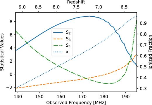
Variance (solid line), skewness (dashed line) and kurtosis (dot–dashed line) of the input light-cone model calculated using all of its pixels as a function of frequency and redshift. The ionized fraction of the model at each redshift is shown as the dotted line. The left y-axis shows corresponding statistical values, whereas the right y-axis shows the ionized fraction. These measurements illustrate the redshift evolution of one-point statistics and act as references for our analysis.
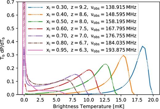
Brightness temperature PDF of the 21 cm light-cone sky model from xi = 0.3–0.8, at every 0.1 step, and at xi = 0.95 ionized fraction. The shape of the PDF changes from Gaussian-like to bi-modal to delta-like function as reionization progresses and manifest the redshift evolution of the statistics shown in Fig. 1.
When discussing the detectability of one-point statistics in the following sections, it will be convenient to characterize the evolution of the statistics at these three characteristic times. For our sky model, they correspond to frequency ranges of ≲160, ∼170–190 and ∼190–195 MHz, respectively. When HERA angular resolution is taken into account, these features will be weakened, and the corresponding frequency might be shifted, but the rise of skewness and kurtosis near the end of reionization along with the negative kurtosis during the bi-modal transition of the PDF will remain as strong indicators of non-Gaussianity in 21 cm signal as we will show in the following sections.
It is also important to note that images from HERA observations will have zero mean as a radio interferometer cannot measure the total power of the sky. Thus, the PDF derived from actual observations will be centred around zero. With angular resolution smoothing, the resulting PDF will be similarly blurred, but the basic evolution of the one-point statistics will persist as they are measured relative to the mean of the signal.
2.4 Mock observations
To simulate mock observations of HERA as described in Section 2.1, we first smooth our sky model with a Gaussian kernel with a full width at half-maximum (FWHM) corresponding to the angular resolution of each of the HERA build-out stages. Then, we pre-allocate 200 non-overlapping fields across the sky project, each field to the instrument observed sine coordinates and measure variance, skewness and kurtosis, using only pixels within a radius equal to half of an FWHM of the HERA primary beam from the field centre. Before calculating statistics, each field is subtracted by its mean value to emulate the absence of the mean value of the sky in interferometric observations. Then, we randomly select 20 measurements and use their mean as an estimate for statistics recoverable by an HERA drift scan. To estimate the sample variance of the drift scan, we repeat the random draw of the 20 measurements, calculate the drift scan estimate from each draw, and use the standard deviation of all estimates as the drift scan sample variance uncertainty. In addition, we use the standard deviation of all 200, single-field, measurements as an estimate for the single field sample variance uncertainty, and statistics calculated from all pixels of the sky model smoothed to HERA angular resolution as the estimate of the ideal signal.
We assume tint = 100 h for every Δν = 80 kHz spectral channel as discussed earlier. The number of samples per measurement in a observation will be limited by the field of view and the angular resolution of the telescope. Because our maps oversample the angular resolution with multiple pixels, we calculate the number of independent resolution elements per pixel from the ratio of the pixel and the resolution element areas, fs = ΔΩpix/ΔΩres, and multiply this factor to the number of pixels in a measurement to obtain N. The oversampling of the angular resolution does not affect the statistics because the oversampling factor is cancelled out in the moment equation (see equation 5).
Table 1 summarizes the parameters of our mock observations, where we refer to HERA240 and HERA350 arrays without their outriggers as HERA240 Core and HERA350 Core, respectively.
Instrument specifications for the HERA build-out stages used in our mock observations. We perform the simulation over ∼56 MHz bandwidth, from ∼139 to 195 MHz, with 80 kHz spectral channel bandwidth. Further information on the array configurations can be found in DeBoer et al. (2017).
| Simulation Parameters | HERA19 | HERA37 | HERA128 | HERA240 Core | HERA350 Core |
|---|---|---|---|---|---|
| Collecting area (m2) | 2 925 | 5 696 | 19 550 | 33 405 | 50 953 |
| Maximum baseline (m) | 70 | 98 | 182 | 238 | 294 |
| Angular resolution (deg) | ∼1.53–2.16 | ∼1.10–1.54 | ∼0.59–0.83 | ∼0.45–0.63 | ∼0.37–0.51 |
3 RESULTS
In this section, we present one-point statistical measurements from the simulated observations. We will first show images of the mock observations and present measurements from the HERA350 Core simulation with 80 kHz channel bandwidth. Then, we will investigate if sensitivity could be further improved with bandwidth averaging.
3.1 Simulated observations
Fig. 3 shows simulated observations at xi = 0.5, 0.7 and 0.95 for all of the HERA build-out stages with all panels taken from the same field in our sky model. The angular resolution increases as the telescope grows and the fluctuations become more pronounced. Fig. 4 shows a cut along the frequency direction from the same field at HERA350 Core angular resolution to illustrate the light-cone evolution. The size scale along the frequency direction grows as reionization progresses and reaches a typical size of ∼4 MHz near the end of reionization. The brightness temperature scale of the observed maps is centred around zero with both negative and positive values due to the lack of mean measurements.
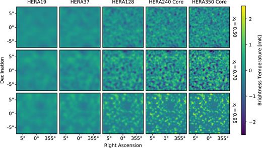
Simulated observations at ionized fraction of 0.5, 0.7 and 0.95 (top to bottom rows) with different HERA build-out stages (left-to-right columns). The 21 cm light-cone model is smoothed to the resolution of each array, showing more pronounced fluctuations as the angular resolution increases. No thermal noise is included in the simulation.
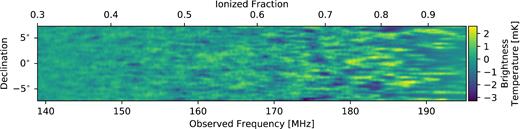
Light-coneslice from the HERA350 Core mock observations. The size scale along the frequency direction grows as reionization progresses and reaches a typical size of ∼4 MHz near the end of reionization.
3.2 HERA350 core measurements
Fig. 5 shows drift scan measurements derived from HERA350 Core simulation with 80 kHz bandwidth, an example of single field measurements, and statistics of the sky model smoothed to HERA350 Core angular resolution. Comparing the drift scan measurements with the input model statistics in Fig. 1, we see the effect of HERA's relatively poor angular resolution, which acts to smooth the input maps, reducing the observed variance, skewness and kurtosis. We will see below that this effect is especially pronounced for the HERA build-out phases, where the coarser angular resolution is predicted to yield one-point statistics that are only weakly non-Gaussian (Mondal et al. 2015).
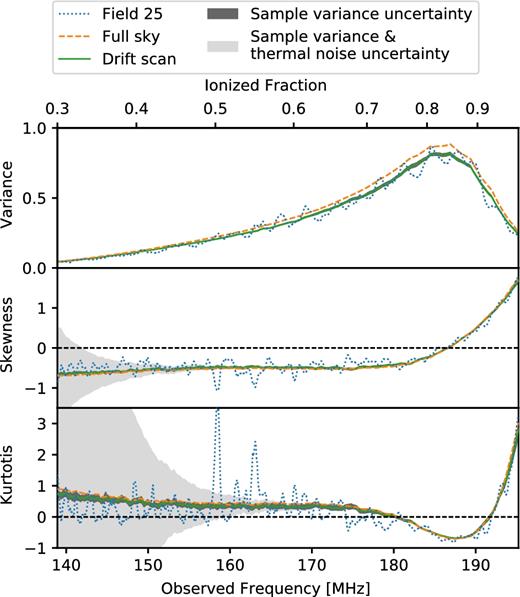
Variance, skewness and kurtosis (top-to-bottom panels) measured from simulated HERA 350 Core observations with 80 kHz channel bandwidth as a function of observing frequency and ionized fraction. The dotted line shows an example of statistics measured from a single field. The solid line shows the drift scan measurements, defined as the mean of 20 single-field measurements. The dashed line shows statistics derived from the full sky after smoothing to HERA350 Core angular resolution as a reference. The two shaded regions show sample variance uncertainty (dark), which is only clearly visible in the kurtosis, and the combined sample variance and thermal noise uncertainty (light) calculated in quadrature for drift scan measurements. HERA350 Core will be sensitive to one-point statistics, particularly in the second half of reionization. Skewness and kurtosis measurements are limited by thermal noise early in reionization and by sample variance later in reionization, while both thermal noise and sample variance are insignificant in variance measurements.
Nevertheless, it is evident that HERA350 Core will be sensitive to one-point statistics, particularly in the second half of reionization where the rise of skewness and the pronounced negative dip and rise of kurtosis indicate non-Gaussian fluctuations. Uncertainty from thermal noise in skewness and kurtosis measurements is large at the beginning of reionization and decreases as frequency increases, becoming negligible in comparison to sample variance at the end of reionization, beyond ∼170 MHz for our sky model. The result is that skewness and kurtosis measurements are limited by thermal noise early in reionization and by sample variance later in reionization. For variance measurements, both thermal noise and sample variance are insignificant and should allow high-sensitivity measurements.
As expected, statistics from single field measurements exhibit fluctuations due to sample variance as opposed to the smoothly evolving ensemble statistics derived from the full-sky model. The fluctuations are interesting in their own right, and we explore their behaviour in Section 4. The 20-field averaged, drift scan observations provide a much more faithful recovery of the model statistics.
3.3 Improving sensitivity with bandwidth averaging
We have only considered measurements from mock observations with 80 kHz channel bandwidth in Section 3.2. The narrow channel bandwidth limits thermal noise performance in the measurements. In this section, we introduce two methods of bandwidth averaging, a commonly used ‘frequency binning’ and a less-common method, mainly used in the 21 cm power spectrum measurements that we term ‘frequency windowing’.
Frequency binning improves thermal noise uncertainty and can be done by averaging maps of neighbouring spectral channels to produce a single output map with larger effective channel bandwidth and lower thermal noise. This is an effective strategy to improve thermal noise until the bin size becomes larger than the typical size of the features in the signal, at which point further increasing the bin size will diminish the strength of the signal by averaging over uncorrelated regions.
We find in Section 3.2 that measurements of one-point statistics by HERA will be constrained by sample variance at high frequencies towards the end of reionization, rather than by thermal noise. Frequency binning will not improve sample variance sensitivity because the number of samples that can be used in a measurement is the same for both the binned and un-binned maps when observing over the same field with the same instrument. Thus, it is of interest to explore an additional approach aimed at reducing sample variance. Since sample variance depends on the number of samples per map, which is fixed by the angular resolution and the field of view, the only way to increase the number of samples used in an estimate is to use maps from multiple spectral channels as a single data set. In this method, we form a three-dimensional data cube from multiple maps of neighbouring spectral channels and measure the statistics of the cube, using all samples within the field of view. We term this process frequency windowing. Thermal noise per pixel is unchanged with frequency windowing because the native spectral channel is preserved, but thermal noise uncertainty on the one-point statistic estimates will still decrease due to the 1/N factor in the estimator variance equations (see equations 8–10).
To explore the relative trade-offs between the two methods, we perform frequency binning and frequency windowing on the brightness temperature maps from our HERA350 Core simulation, varying bin and window sizes from 1 to 8 MHz with 1 MHz increment. We start from the highest spectral channel in our ∼60-MHz bandwidth, at 195 MHz, and bin or window, progressing down to lower frequencies. The process is repeated on all 200 sample fields. Then, we make drift scan measurements and estimate thermal noise and sample variance uncertainties for each case using the same method as described in Section 2.
The observed variance decreases across the observed frequency range when frequency binning is used, with particularly rapid decline near the variance maxima. This is expected as the signal strength along the frequency dimension in our HERA350 Core mock observations, shown in Fig. 4, is smaller and more uniform early in reionization but grows and reaches the maximum strength and maximum variance at around 185 MHz. Binning the signal when both the signal strength and signal variance are high will greatly reduce the signal amplitude, resulting in much smaller observed variance. As a side note, the observed variance only slightly declines between the native 80-kHz channel bandwidth and 1-MHz binning case. This is expected as the coherence length of the 21 cm signal is predicted to be approximately 1 MHz (Santos, Cooray & Knox 2005). Thus, the bin size finer than 1 MHz would not dramatically alter the signal variance. Although not shown, we find that the overall evolution of skewness and kurtosis recovered by the instrument do not change when frequency binning is used apart from slight variations between bins.
Compared to frequency binning, frequency windowing simply adds more samples along the frequency dimension. With no averaging of maps from neighbouring spectral channels, variance of the signal within each spectral channel is preserved, and the observed variance would be the mean value of variance of all spectral channels within that window. Skewness and kurtosis are also preserved as the added samples from neighbouring spectral channels do not alter the shape of the PDF but contribute to form a more well sampled PDF, unless strong redshift evolution occurs between spectral channels. All statistics measured from frequency windowing data also show less variation between window to window and follow the sky model more closely.
We find that frequency windowing improves the sensitivity more than frequency binning at nearly all redshifts in our simulations since sample variance dominates the uncertainty over much of the modelled band. To illustrate, we compare in Fig. 6 the signal-to-noise ratio (SNR) of the statistics for different binning and windowing cases measured from the HERA350 Core simulation. We calculate SNR by dividing the absolute values of statistics with the square root of the quadrature sum of thermal noise uncertainty and sample variance uncertainty. As evidence from the figure, SNR of variance and skewness are much improved when frequency windowing is used, especially with larger window sizes. In contrast, frequency binning only improves SNR at higher redshift where thermal noise dominates the uncertainty and larger frequency bins yield lower thermal noise. However, this improvement stops after the bin size reaches a few MHz because thermal noise has been reduced below sample variance at that point, putting the measurements in sample variance limited regime. With frequency windowing, SNR continues to improve with larger windows. Although we only investigate up to an 8-MHz window case, we expect further improvement beyond the 8 MHz window. However, redshift evolution will have detrimental effect on the signal with that large bandwidth; thus, the logical choice would be to perform frequency windowing only with a large enough window size to obtain sufficient SNR.
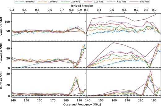
Comparing SNR measured from HERA350 Core simulation with different frequency binning (left column) and frequency windowing (right column) cases. SNR is defined as the ratio of the absolute values of statistics and the square root of the quadrature sum of thermal noise uncertainty and sample variance uncertainty. Frequency windowing improves the sensitivity more than frequency binning at nearly all redshifts due to the reduced sample variance.
We must note that mathematically predicting the trend of the SNR improvements from frequency windowing is challenging because sample variance is signal dependent and depends on several factors. Our results in Fig. 6 show no correlation between SNR improvements and the window size, and the improvements appear to be frequency-specific. With frequency windowing, skewness shows the maximum increases in the SNR at xi ≈ 0.5 while kurtosis SNR is the most improved at xi ≈ 0.85, in the negative kurtosis regions. Since frequency windowing does not change the statistics, the difference in SNR improvements must depend on the underlying nature of the signal.
3.4 Performance of HERA build-out stages
Although it is clear from Sections 3.2 and 3.3 that the complete HERA 350 Core array will be able to mitigate sample variance by averaging statistics measured over multiple fields across the sky and utilizing frequency windowing, it is important to see how the smaller, planned built-out, arrays will perform as data from HERA 350 Core will not be available until after 2020.
In general, smaller arrays have two key disadvantages of less collecting area and worse angular resolution. Typically, smaller collecting area increases the thermal uncertainty, while poorer angular resolution smooths over the intrinsic 21 cm features, yielding a more-Gaussian like signal with lower amplitude than for higher angular resolutions. However, HERA is very close to being a filled aperture array, resulting in the angular resolution and array collecting area that roughly scale as the maximum baseline and the maximum baseline squared, respectively. As a consequence, it can be shown from equation (7) that the thermal uncertainty per resolution element of HERA does not change with the size of the array. Thus, the only disadvantage of smaller HERA array is the reduced angular resolution that damps the signal and lowers the number of independent resolution elements per map.
For a detailed investigation, we perform frequency binning and frequency windowing on the mock observations of all HERA build-out stages, and calculate the mean drift scan statistics, sample variance uncertainty and thermal noise uncertainty for each case following the methods described in Section 2.4. The HERA build-out arrays cover angular resolution from ∼1.5 deg to 0.5 deg as the array grows. Thus, this study also gives an insight into the effects of angular resolution on the one-point statistics.
Fig. 7 shows the one-point statistics measured from the mock observations of each of the build-out stages, along with the corresponding SNR calculated in the same manners as in Section 3.3, with 4 MHz frequency windowing applied before the calculations. It is clear that the derived statistics are affected by the increasing angular resolution as the array grows. Variance decreases with smaller arrays, similar to the effect of frequency binning. Skewness and kurtosis measured from smaller, HERA19 and HERA37, arrays also vanish, only fluctuating near zero throughout much of reionization. In contrast, the larger HERA128, HERA240 Core and HERA350 Core arrays exhibit non-zero skewness and kurtosis even early in reionization, diverging more from zero as the angular resolution improves. The negative region of kurtosis near the end of reionization only reaches significance in observations with these large build-out phases.
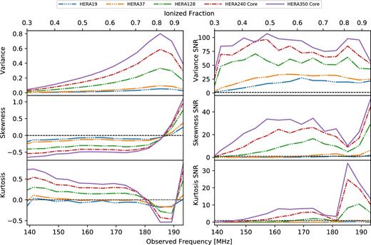
Drift scan statistics (left) and SNR (right) measured from the mock observations of all planned built-out HERA stages with 4-MHz frequency windowing applied before the calculations. All HERA configurations should be able to measure the variance with high SNR. In addition, HERA128 and above will be able to measure the characteristic rise of skewness and the dip, then rise, of kurtosis near the end of reionization with sufficient SNR.
This resolution effect is an expected consequence from the angular resolution smoothing. With finer angular resolution, larger HERA arrays can resolve more of the intrinsic underlying fluctuation and preserve the amplitude of the signals. The shape of the PDF distribution of the signal is also preserved, and thus the values of skewness and kurtosis remain closer to the intrinsic level of the signals. When the angular resolution becomes larger than the typical sizes of the underlying signals, angular resolution smoothing blurs out the fluctuations, reduces the overall signal amplitude and shift the PDF from non-Gaussian to Gaussian. As a result, variance is greatly reduced, and skewness and kurtosis vanish. These results are in agreement with Mondal et al. (2015), who suggests, based on the study of 21 cm power spectrum SNR, that 21 cm signal would only be weakly non-Gaussian at a degree scale near the end of reionization, comparable to angular resolution of HERA19 and HERA37 arrays, and be mostly Gaussian otherwise.
Apart from better resolving the intrinsic fluctuations, increasing the angular resolution will also reduce sample variance. However, the signal-dependent nature of sample variance is still true. Thus, we see the same frequency-specific SNR improves as the array grows in size similar to the SNR improvement from frequency windowing as the window size grows (see Fig. 6). All statistics measured from the mock observations of the arrays with finer angular resolutions also show less variation between window to window and follow the sky model more closely.
Our simulations suggest that all HERA configurations should be able to measure the variance with high SNR. In addition, HERA128, HERA240 Core and HERA350 Core will be able to measure the characteristic rise of skewness and the dip, then rise, of kurtosis near the end of reionization with sufficient SNR, especially when frequency windowing is used, as demonstrated in Fig. 7.
4 INDIVIDUAL FIELD OBSERVATIONS
In this paper, we focus on recovering the one-point statistics over multiple fields corresponding the full drift scan area that will be surveyed by HERA. Here, we briefly turn our attention to the individual 9 × 9 deg2 HERA beam fields in our simulations. As expected, statistics measured within individual fields are more susceptible to sample variance. For example, there are two strong kurtosis spikes near 160 MHz in the measurement from field number 25 from our HERA350 Core simulation as shown in Fig. 5. These kurtosis spikes are factors of 7 and 5 above the sample variance expected for the field. Significant outlier deviations such as these are seen in fields with one or two large cold or hot spots. Fig. 8 illustrates the case. When cold or hot spots appear in the observed fields, they perturb the PDF, adding more density to the tails of the distribution, and causing kurtosis to rise. In some occasions, these outliers also shift the symmetry of the PDF and cause strong troughs in the skewness as appeared in Fig. 5. Outlier one-point statistics of small fields may provide a simple and robust bubble detector and a new tool to constrain reionization models. Statistical study of the frequency of occurrence of the outlier kurtosis (or skewness) peaks could be conducted for a given instrument and related to predictions from reionization models. The outliers should be less susceptible to noise in the underlying fluctuations than typical estimates of the statistics. Investigation of this possible metric would require further study that is beyond the scope of this work.
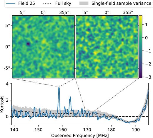
Illustrating the correlation between strong sample variance fluctuation in the single-field measurement of kurtosis and the outlying cold or hot spots in the observed field. The bottom panel re-draws the kurtosis measured from field 25 as in Fig. 5, overlaid on top of a 1σ single-field sample variance uncertainty plotted around the mean of kurtosis measurements from all fields. The top two panels show maps of the underlying brightness temperature signal at ∼158 MHz, where the kurtosis rises above the sample variance uncertainty (left), and at ∼170 MHz, where the kurtosis is near zero (right). The outlying cold spots perturbs the tail of the PDF, causing kurtosis to rise. This statistical feature could potentially be used as a bubble indicator.
5 CONCLUSION
We have established a baseline sensitivity analysis of 21 cm one-point statistics from the EoR for HERA through realistic mock observations of redshifted 21 cm brightness temperature fluctuations.
We develop a tile-and-grid method that transforms a suite of small 21 cm simulation cubes into a full-sky light-cone input model that matches the dimensionality of the observational data. We incorporate the angular resolution effects of all of the planned build-out stages of HERA to gauge the sensitivity of the array as it grows in size. We use simple Gaussian smoothing to incorporate the array angular resolution, using multiple kernel sizes that match angular resolutions of the different build-out stages. The span of resolutions also allows us to study their effects on the statistics. Apart from the variance and skewness that have extensively been covered in previous studies, we also measure kurtosis from our mock observations as well as deriving sample variance uncertainty associated with the measurements. Uncertainty from thermal noise is mathematically derived from the framework developed in Watkinson & Pritchard (2014), where we have extended their derivation to kurtosis. We calculate SNR to gauge the sensitivity of the measurement and perform frequency binning and frequency windowing to investigate if the sensitivity can be further improved. We ignore foreground contamination and other systematics in this work, postponing them to future works.
Our results show that measurements of 21 cm one-point statistics by HERA will likely be limited by sample variance, at least near the end of reionization. Particularly, the variance sensitivity is sample variance limited throughout reionization while skewness and kurtosis sensitivities will be limited by thermal noise early in reionization and by sample variance later in reionization. Frequency windowing can be used in all measurements to improve the sensitivity. However, care must be taken to not use a window size that is too large to avoid redshift evolution. In addition, all build-out stages of HERA will be able to measure variance with high sensitivity, and HERA128 and above will also be able to measure skewness and kurtosis.
An introduction of kurtosis into our analysis has led us to identify kurtosis peaks as potential indicators of outlying cold or hot spots in individual fields of observations. Kurtosis will sharply rise when a few hot or cold outlying regions appear on top of the underlying Gaussian-like signal in the observed field. Further investigation of this feature is beyond the scope of this work.
Although we only focus on HERA in this paper, our results should be applicable to future arrays such as the SKA. In particular, sample variance uncertainty will be further improved due to its higher angular resolution.
There are three main obstacles in pursuing future detection and characterization of the EoR with 21 cm one-point statistics: (1) the sensitivity of existing reionization arrays to the statistics, (2) mitigation of astrophysical foreground contamination, and (3) estimation of reionization parameter constraint from the statistics. We have extensively covered the first point in this paper, focusing on the HERA array, and we are actively investigating the effects of foreground contamination on our results. The last point is arguably the least well-understood, and we will investigation the topic in the future.
Acknowledgements
This work is supported by the U.S. National Science Foundation (NSF) award AST-1109156. P.K. is supported by the Royal Thai Government Scholarship under the Development for Promotion of Science and Technology Talent Project. DCJ is supported by an NSF Astronomy and Astrophysics Postdoctoral Fellowship under award AST-1401708. APB is supported by an NSF Astronomy and Astrophysics Postdoctoral Fellowship under award AST-1701440. NT is a Jansky Fellow of the National Radio Astronomy Observatory.
Footnotes
In statistics, the precise term of this definition is excess kurtosis, which subtracts 3 from the standard definition of kurtosis, m4/(m2)2, to yield zero kurtosis for Gaussian distribution. Here, we simply use kurtosis to refer to excess kurtosis.
REFERENCES
APPENDIX A: FULL-SKY light-cone
The observable sky at a particular redshift is a sphere in comoving space. No existing 21 cm simulation spans a volume large enough to contain the whole observable sky at the redshifts of interest for reionization. The typical size of a large 21 cm simulation box presently is ∼2 Gpc while a comoving distance to redshift 8.5 (νobs ≈ 150 MHz) is ∼9.3 Gpc. To create a full-sky 21 cm model, we exploit the periodic boundary condition of the 21 cm simulations and effectively tile the simulation volume in comoving space to obtain a sufficiently large volume before gridding on to the sky sphere. The process is repeated at each redshift of interest to create maps for the full light-cone. Fig. A1 shows a schematic diagram of our tiling and gridding process.
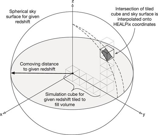
Schematic diagram illustrating the tiling of simulation cubes with periodic boundary conditions to produce a full-sky light-cone. The diagram shows the process for a single redshift. The process is repeated for every observed redshift using an evolved simulation cube for each redshift and the appropriate comoving distance diameter for each redshift. The (x, y, z) coordinates in the diagram represent both the comoving coordinates of the simulation cubes and the Cartesian coordinates of the HEALPix sphere.
We start with a suite of theoretical 21 cm cubes from the semi-analytic simulations of Malloy & Lidz (2013). The cubes span the redshift range 9.3 > z > 6.2, with Δz = 0.1 steps, representing the universe from ∼ 30 per cent to 96 per cent ionized. The simulation volume is 1 Gpc3 in a 5123 pixel box with periodic boundary. We linearly interpolate the simulated 21 cm cubes across redshift to produce new cubes that more-closely match the redshifts observed by HERA in steps of 80 kHz spectral channels between ∼139 and 195 MHz. The interpolation step is not required to construct the light-cone if simulation cubes matching the redshift of interests are available. For each of the redshifts, we tile the interpolated cube with itself in three dimensions to construct an arbitrarily large simulated volume for that redshift. Then, we draw an observable sky at that redshift as a sphere of radius equal to the comoving distance of that redshift from a fixed origin inside the volume and interpolate the nearest neighbouring pixel from the cube to the corresponding HEALPix pixel location on the sphere. Before tiling and gridding, we degrade each simulation cube to 1283 box to reduced computing time while retaining all size scales that can be probed by HERA. We use HEALPix pixel area that is ∼10 times smaller than the resolution of the simulations (NSIDE = 4096) to avoid sampling artefacts. This process is repeated for every observed redshift to produce a suit of full-sky maps that accurately represent the redshifted 21 cm light-cone model.
Compared to flat-field approximations for tiling and gridding that do not take into account the spherical surface of the sky, our method is equivalent to slicing a simulation cube from different angles and rotational axes and mapping the slices on to a sphere at different locations. Thus, even within the ∼9 deg HERA fields, we see significantly reduced repetition of spatial structure in the resulted maps in comparison to the flat-field approximation. Fig. A2 illustrate this point, where we use the method from Zawada et al. (2014) to produce a standard flat-field light-cone cube and compare it with a light-cone cube produced by gridding on to spherical surfaces. The full-sky HEALPix maps produced with spherical surface gridding preserve one-point statistics of the original simulations, showing changes less than 0.001 per cent of the original values for our simulation sets.
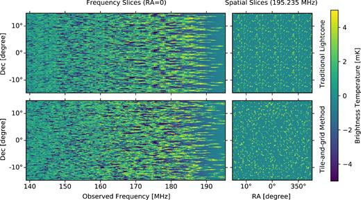
Comparison of flat-field light-cone tiling with our spherical surface projection. Top panel shows the flat-field light-cone and the bottom panel shows the spherical surface light-cone. Even over the relatively small area plotted, repetition of structure is visible in the flat-field light-cone, whereas the spherical surface method results in a random appearance while still preserving the one-point statistics of the original simulation cubes. The flat-field light-cone cube is interpolated from comoving (x, y, z) directly to celestial image coordinates. The two images are identical along Dec = 0 deg row.
APPENDIX B: KURTOSIS UNCERTAINTY PROPAGATION
The method of uncertainty propagation for one-point statistics is first described in Watkinson & Pritchard (2014). Here, we summarize and expand on their work, deriving uncertainty propagation for the kurtosis in addition to variance and skewness.
Additional Gaussian noise identities for derivation of estimator variance of kurtosis. Please see table A1 in Watkinson & Pritchard (2014) for more identities.
| |$\langle n_i n_j^4 \rangle \, \langle n_i^5 \rangle =0 \, (i=j) \langle n_i \rangle \langle n_j^4 \rangle =0 \, (i \ne j)$| | |$\bigg\rbrace 0$| |
| |$\langle n_i^2 n_j^4 \rangle \langle n_i^6 \rangle =15\sigma _i^6\, (i=j) \langle n_i^2 \rangle \langle n_j^4 \rangle =3\sigma _i^2\sigma _j^4 \, (i \ne j)$| | |$\bigg\rbrace (3+12\delta _{ij})\sigma _i^2\sigma _j^4$| |
| |$\langle n_i^3 n_j^4 \rangle \langle n_i^7 \rangle =0 \, (i=j) \langle n_i^3 \rangle \langle n_j^4 \rangle =0 \, (i \ne j)$| | |$\bigg\rbrace 0$| |
| |$\langle n_i^4 n_j^4 \rangle \langle n_i^8 \rangle =105\sigma _i^8 \, (i=j) \langle n_i^4 \rangle \langle n_j^4 \rangle =9\sigma _i^4\sigma _j^4 \, (i \ne j)$| | |$\bigg\rbrace (9+96\delta _{ij})\sigma _i^4\sigma _j^4$| |
We follow the procedure in Watkinson & Pritchard (2014) and are able to confirm their results. In addition, we derive the estimator variance for kurtosis as follows.
