Can The Pore Scale Geometry Explain Soil Sample Scale Hydrodynamic Properties?
 Sarah Smet
 Eléonore Beckers1
  Erwan Plougonven
 Angélique Léonard
 Aurore Degré
- 1Soil Water Plant Exchanges, BIOSE, Gembloux Agro-Bio Tech, University of Liège, Gembloux, Belgium
- 2Chemical Engineering, University of Liège, Liège, Belgium
For decades, the development of new visualization techniques has brought incredible insights into our understanding of how soil structure affects soil function. X-ray microtomography is a technique often used by soil scientists but challenges remain with the implementation of the procedure, including how well the samples represent the uniqueness of the pore network and structure and the systemic compromise between sample size and resolution. We, therefore, chose to study soil samples from two perspectives: a macroscopic scale with hydrodynamic characterization and a microscopic scale with structural characterization through the use of X-ray microtomography (X-ray μCT) at a voxel size of 21.53 μm3 (resampled at 433 μm3). The objective of this paper is to unravel the relationships between macroscopic soil properties and microscopic soil structure. The 24 samples came from an agricultural field (Cutanic Luvisol) and the macroscopic hydrodynamic properties were determined using laboratory measurements of the saturated hydraulic conductivity (Ks), air permeability (ka), and retention curves (SWRC). The X-ray μCT images were segmented using a global method and multiple microscopic measurements were calculated. We used Bayesian statistics to report the credible correlation coefficients and linear regressions models between macro- and microscopic measurements. Due to the small voxel size, we observed unprecedented relationships, such as positive correlations between log(Ks) and a μCT global connectivity indicator, the fractal dimension of the μCT images or the μCT degree of anisotropy. The air permeability measured at a water matric potential of −70 kPa was correlated to the average coordination number and the X-ray μCT porosity, but was best explained by the average pore volume of the smallest pores. Continuous SWRC were better predicted near saturation when the pore-size distributions calculated on the X-ray μCT images were used as model input. We also showed a link between pores of different sizes. Identifying the key geometrical indicators that induce soil hydrodynamic behavior is of major interest for the generation of phenomenological pore network models. These models are useful to test physical equations of fluid transport that ultimately depend on a multitude of processes, and induce numerous biological processes.
Introduction
The development of visualization techniques has played a major role in fully describing soil functions. Serial sectioning, a well-established method (Cousin et al., 1996), has been replaced by replaced by 3D non-destructive visualization techniques are becoming more easily available, with added benefit of less time-consuming procedures that provide higher resolution images (Grevers et al., 1989). However, Roose et al. (2016) have wisely said, “Technological advances alone are not sufficient. Real advances in our understanding will only be achieved if these data can be integrated, correlated, and used to parameterize and validate image based and mechanistic models.” X-ray micro-computed tomography (X-ray μCT) has been widely used in soil science making comparisons between studies possible. (Taina et al., 2008) and Wildenschild and Sheppard (2013) discuss the use of X-ray μCT to study the vadose zone. We also will mention the visual analysis of the air and water distributions within pore spaces, which are both important physical variables for activity of soil biota (e.g., Young et al., 1998; Or et al., 2007; Falconer et al., 2012; Monga et al., 2014; Vogel et al., 2015). One approach is to visualize the soil at high resolution to identify hot-spots of microbial activity (e.g., Gutiérrez Castorena et al., 2016), simulate air-water interfaces within the pore network (e.g., Pot et al., 2015) or quantify the impact of the pore network architecture on the microorganism's activity (e.g., Kravchenko and Guber, 2017). Another approach is to provide a more specific description of the fluid transport capacities (Vogel et al., 2015) which could ultimately improve field-scale models of microbial activity and biochemical processes (Blagodatsky and Smith, 2012). De facto, when dealing with agricultural and environmental properties of the soil, an accurate description and prediction of its transport capacities in the unsaturated state is the overarching goal.
It is well-known that, due to natural or anthropogenic actions, there is quite a range in the variability in fluid transport parameters [e.g., saturated hydraulic conductivity (Ks) or air permeability (ka)] between samples with homogenous textures (Baveye and Laba, 2015; Naveed et al., 2016), due to the uniqueness of the porosity distribution and the connectivity within a sample. Studies have, therefore, focused on the link between the inner pore space structure of a sample and its specific fluid transport properties. On one hand, experimentally visualized infiltration studies shed light on the effective conducting pore network which represents only a small portion of the total network (Luo et al., 2008; Koestel and Larsbo, 2014; Sammartino et al., 2015). The procedures developed in these studies are promising, but restricted to the analysis of large macropores because of the trade-off between resolution and acquisition time. On the other hand, numerical simulations based on pore space are used to predict conductivity. Many studies focused on idealized porous structures (e.g., Vogel et al., 2005; Schaap et al., 2007) and a few deal with actual soil (Elliot et al., 2010; Dal Ferro et al., 2015; Tracy et al., 2015). The latter show encouraging results, but are restricted to a defined resolution and/or sample size (Baveye et al., 2017). Indeed, the direct approach of linking one structure to one function is limited by the difficulty in analyzing the structure in a representative way, so that the soil is adequately characterized (Vogel et al., 2010). The description of soil microscopic structure via global characteristics could encompass that challenge and comparisons of one soil microscopic structure to its own macroscopic properties have indeed gained attention.
Luo et al. (2010) were among the first to measure Ks and the break through curve characteristics on soil samples that were also scanned with X-ray μCT and analyzed in 3D (16 soil cores of 5 × 6 cm and 10.2 × 35 cm and voxel sizes ranging from 2502 × 1,000 μm3 to 12 × 10 mm3). They found that μCT macroporosity, the number of independent macropore, macropore hydraulic radius and angle were identified as the most important microscopic characteristics to explain fluid transport. From 18 soils cores (10 × 9 cm) scanned at a voxel size of 1863 μm3 and 17 soil cores (19 × 20 cm) scanned at 4302 × 600 μm3, respectively, Naveed et al. (2012) and Katuwal et al. (2015b) found that the lowest μCT macroporosity value for any quarter length of sample height adequately explained air permeability (ka) measured at a water matric potential (h) of −3 or −2 kPa, respectively. Paradelo et al. (2016) showed that the minimum value of macroporosity along a sample depth was most correlated to Ks and ka (45 soil cores of 20 × 20 cm and voxel size of 4302 × 600 μm3). Mossadeghi-Björklund et al. (2016) also demonstrated that Ks was significantly correlated to μCT macroporosity within a compaction experiment (32 soils cores of 20 × 20 cm and voxels size of 4302 × 600 μm). Eventually, Naveed et al. (2016) suggested that biopore-dominated and matrix-dominated flow soil cores should be distinguished before analyzing relationships between microscopic and macroscopic soil properties. They indeed found distinct significant power regressions between Ks or ka (measured at h = −3 and −0 kPa) and μCT macroporosity for the two categories of the 65 soil cores (6 × 3.5 cm and voxel size of 1293 μm3). These observed relationships between flow parameters and μCT porosity are actually intuitive, but they depend on image resolution, water matric potential and soil type. For example, Lamandé et al. (2013) did not find the expected relationship between μCT porosity and ka measured at h = −10 kPa, but rather a linear positive relationship between the number of pores and ka (32 soil cores of 19 × 20 cm and voxel size of 6003 μm3). Finally, Anderson (2014) found that Ks could reasonably be estimated from the μCT number of pores and the μCT macroporosity fractal dimension (336 soil cores of 7.62 × 7.62 cm and voxel size of 0.192 × 0.5 μm3).
The μCT porosity, number of pores, average pore radius, surface area, and pore network connectivity and tortuosity all depend on the minimal visible pore size, in other words, on the resolution of the binary X-ray μCT images used to obtain the pore network (Houston et al., 2013; Peng et al., 2014; Shah et al., 2016), additionnaly, useful information about conducting pores is lost with increased voxel size. One strategy to minimize this limitation is to use grayscale information. Crestana et al. (1985) demonstrated a linear dependence between the gray value of the soil matrix in Hounsfield unit (HU) and the soil water content. More recently, Katuwal et al. (2015a) found the CT number of the soil matrix (average grayscale value in HU) as a useful descriptor for determining the magnitude of preferential flow, and Paradelo et al. (2016) showed that global macroporosity values combined with the CT-matrix number best explained the variation in air and water transport parameters. Another strategy would be to scan soil samples at higher resolutions. For example, Sandin et al. (2017) worked at a voxel size of 1203 μm3 and observed significant correlations between Ks and a global measure of the pore network connectivity (from the percolation theory) which had, to our knowledge, never been observed (20 soil samples of 6.8 × 10 cm). Pore network connectivity and tortuosity are important indicators of flow capacities (Perret et al., 1999; Vogel, 2000). There is still a lack of information on the links between global pore network complexity indicators and flow parameters. It is indeed challenging to identify and describe the part of the conducting pore network that dominates flow. We, however, hypothesize that it might come from the resolution at which previous studies were performed.
Within that context, the objectives of this study are to: (i) characterize the microscopic structure of twenty-four soil samples at a resolution of 21.5 μm resampled to 43 μm; and (ii) explore the relationships between soil microscopic characteristics and its saturated hydraulic conductivity, air permeability and retention capacities using Bayesian statistics.
Materials and Methods
Soil Sampling
Twenty-four vertical undisturbed soil samples (3 cm in diameter and 5 cm in height) were taken at the surface of an agricultural soil in Gembloux, Belgium (50°33′N, 4°42′E). According to the WRB soil system (2006), this soil is classified as a Cutanic Luvisol with an average of 14.3% of clay, 78.3% of silt and 7.4% of sand. This type of soil is representative of the intensive central agricultural area in Belgium. Sampling was performed 24 to 48 h after a rain. In order to minimize sampling disturbance, the plastic cylinders were manually driven into the soil until the top of the cylinder was at the surface level and then manually excavated.
Macroscopic Measurements
Soil samples were first upward saturated with distilled water. Their characteristic soil water retention curve (SRWC) was then measured using pressure plates (Richards, 1948; DIN ISO 11274, 2012). After being weighed at a water matric potential of −7, −10, −30 and −70 kPa, the air permeability of the samples was measured by applying an air flow across the sample and measuring the resulting inner-pressure with an Eijkelkamp air permeameter 08.65 (Eijkelkamp Agrisearch Equipment, Giesbeek, The Netherlands). As recommended by the constructor, each measure was repeated five times and kept as short as possible. Corey's law was then applied to calculate the air permeability [L2] (Corey, 1986 in Olson et al., 2001). At −70 kPa, the soil samples were scanned using an X-ray microtomograph (see next section) before the end of their SWRC was measured (water matric potential of −100, −500, and −1500 kPa). After reaching −1,500 kPa, the soil samples were saturated once again and the saturated hydraulic conductivity (Ks [LT−1]) was measured using a constant head device (Rowell, 1994) and applying Darcy's law. Finally, the soil samples were oven-dried at 105° for 7 days to obtain their dry weight. Porosity [L3L−3] was calculated as the ratio between the volume of water within the saturated soil sample and its total volume (McKenzie et al., 2002). From McKenzie et al. (2002), the bulk density (BD) [ML−3] was deduced from the porosity value (PO) assuming a particle density of 2.65 g/cm3.
Microscopic Measurements
Image Acquisition
After reaching a water matric potential of −70 kPa, the soil samples were scanned using a Skyscan-1172 desktop micro-CT system (Bruker microCT, Kontich, Belgium). The choice of scanning parameters (filters, number of projections, 180 or 360°, projection averaging) was made by evaluating reconstruction quality over acquisition time. The X-ray source was set at 100 kV and 100 μA and an aluminum-copper filter was used to reduce the beam hardening artifacts in the reconstruction. The rotation step was set at 0.3° over 180° and, to improve the signal-to-noise ratio, the average of 2 projections was recorded at each rotation step. The exposure time was 600 ms. The field of view was 21 × 14 mm and, to cover the entire sample, a 2 × 4 grid of sub-regions were scanned (in the Skyscan software this corresponds to using both the “wide image” mode and “oversize scan” mode). Given these parameters, the total acquisition time was ~4 h. We adjusted the detector configuration (16-bit X-ray camera with 4 × 4 binning, creating 1000 × 666 pixel radiograms) and the distance between the camera and the soil sample in order to obtain radiographs with a pixel size of 21.5 μm.
Image Processing
Tomographic reconstruction was performed with the NRecon® software, freely provided by Brüker. Automatic misalignment compensation was used along with a level 7 (out of 20) ring artifact correction. No beam hardening post-corrections were applied. The lower limit for the histogram grayscale range was set at zero, as recommended by Tarplee and Corps (2008). The upper limit, the same for all samples, was the maximum value between the automatically generated upper limit for each sample. After reconstructions, the 3D images were cropped to only select the volume within the sampling cylinders (radius of 700 pixels) and the image's contrast was improved in Matlab (MathWorks, UK).
Prior to segmentation, a 3D median filter with a radius of 2 pixels was applied to the images to decrease noise (Smet et al., 2017). Because of computational cost, sub-sampling was performed and the final voxel size was 43 μm in all directions. This process follows recommendation from Houston et al. (2013) and Shah et al. (2016), which is to scan a sample at the highest possible resolution even if a post-scan coarsening is necessary. We then applied the global porosity-based segmentation method developed by Beckers et al. (2014b). To that purpose, we firstly calculated the potential maximal visible pore size from capillary law and voxel size information (433μm3). Then, from the laboratory SWRC data, the potential visible porosity for each soil samples was obtained; it was the air-filled porosity at h = −1 kPa (equivalent radius of 150 μm). The porosity-based segmentation method selects an initial global threshold with Otsu's method (Otsu, 1979), and then compares the porosity of the resulting binary image (ratio of pore voxels over the total amount of voxels) to the estimated soil sample visible porosity. Through an iterative loop, the threshold is then adjusted to minimize the difference between this calculated porosity and the estimated soil sample visible-porosity. This method has been proven satisfactory (Beckers et al., 2014b; Smet et al., 2017) and the Matlab R2015a (MathWorks, UK) code was provided by the authors. Finally, a visual inspection was performed to evaluate the segmentation quality and, in case the porosity-based segmentation method failed, Otsu's segmentation was used. A post-segmentation cleanup was applied to remove any pores smaller than five voxels.
Quantification of Soil Microscopic Features
After segmentation, the images were imported into Avizo where codes developed by Plougonven (2009) were used. Those codes provide a 3D morphological quantification of the pores based on the skeleton where a pore is defined as “part of the pore space, homotopic to a ball, bounded by the solid, and connected to other pores by throats of minimal surface area” (Plougonven, 2009), the pore boundaries are demarcated by the local geometry. The resulting 3D quantification information regarding pores chambers connected by pores throats included pore localization, volumes, specific surface, connected surfaces, number of connections, deformation and inertia tensor. From those data, we calculated several microscopic parameters (Table 1) as well as the pore-size distribution with radius calculated from the assumption that pores were elliptic cylinders (Beckers et al., 2014a). After morphological processing in Avizo, we imported the binary images in ImageJ (Schneider et al., 2012) where the BoneJ plugin (Doube et al., 2010) functionalities were used; all the measurements into ImageJ were performed in 3D. The skeletonisation tool was used to find the pore's centerline and extract a skeleton made of branches that are connected by junctions. It was achieved by external erosion with a 3D medial axis thinning algorithm. All the calculated microscopic parameters presented in Table 1 are commonly used in studies regarding the use of X-ray in soil science. We calculated the large porosity (Large_PO) in order to be comparable to the results discussed in the introduction of this paper where the voxel size was ~10 times larger.
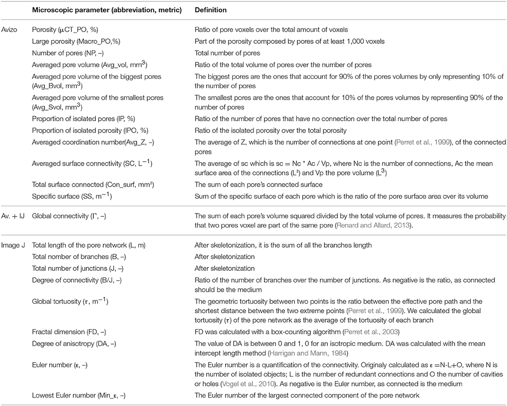
Table 1. Calculated microscopic parameters on the X-ray μCT images and their definition.
3D Visualization
In order to obtain clear 3D representations, all 24 soil X-ray μCT images were subjected to the following process: any pore that was not part of the largest connected component was removed using the MorphoLib plugin (Legland et al., 2016) in ImageJ (Schneider et al., 2012), a cylindrical region of interest of 295 pixels in radius was then used to remove the edge effects caused by sampling with the initial height going unchanged. Visualization was performed using the 3DViewer plugin (Schmid et al., 2010) in ImageJ (Schneider et al., 2012).
Results Analysis
Basic descriptive statistics were performed on the macroscopic and microscopic data. The correlation coefficients (ρ) between the different microscopic parameters were then calculated using Bayesian statistics (see next section) to account for data uncertainty. Then, Bayesian correlation coefficients were calculated between relevant microscopic and macroscopic measurements as well as Bayesian linear regression models. Before implementation, the data were randomly split into calibration (18 soil samples) and validation (6 soil samples) sets. To that purpose, a number was assigned to each of the 24 soil samples and six numbers were randomly picked. Therefore, the soil samples have a sequential numbering. The calibration set includes samples from #1 to #18 and the validation set from #19 to #24.
Bayesian Statistics for Correlation and Linear Regression
When a linear relationship was visually assumed between two variables, the correlation coefficient between those two variables was calculated using Bayesian statistics. In Bayesian statistics a probability is assigned to a model [P(observations|model)] rather than to an observation, as in frequentist statistics. From the observations, the models (the prior) are updated to posterior distributions [P(model|observations)] and the uncertainty of the statistic description is expressed in a probabilistic way through the posterior distributions parameters. We refer to Marin and Robert (2007) for more information about Bayesian statistics. In this study, we used the package “BayesMed” (Nuijten et al., 2015) in R (R Core Team, 2015), which computes a Bayesian correlation test, the null hypothesis (H0) being that the correlation coefficient is null. The correlation test is based on a linear regression between two variables with a Jeffreys-Zellner-Siow (JZS) prior as a mixture of g-priors (Liang et al., 2008; Wetzels and Wagenmakers, 2012). The correlation coefficient is extracted from the posterior variance matrix. We computed the test without expectation about the direction of the correlation effect (Wagenmakers et al., 2016). The credibility of the test is assumed by comparing the marginal likelihoods of the regression model to the same regression model without the explaining variable (Bayes Factor, BF), which quantify the evidence for one or the other hypothesis. Another advantage of using the Bayesian approach is the possibility of quantifying the evidence for the null hypothesis (Wetzels and Wagenmakers, 2012). Non-significant tests in frequentist statistics are interpreted in favor of the null hypothesis although the result could be induced by a noisy data set. Therefore, because the posterior distributions are updated from the observations, the conclusion of the test will not depend on the number of observations and it is possible to recalculate BF as the observations are logged-in and stop the collect when the evidence is compelling. Adapted from Jeffreys (1961) in Wetzels and Wagenmakers (2012), BF's larger than 100 were interpreted as decisive evidence for H1; BF's between 30 and 100 as a very strong evidence for H1, BF's between 10 and 30 as a strong evidence for H1, BF's between 3 and 10 as a substantial evidence for H1 and BF's below 3 as an anecdotal evidence for H1. The values of BF's that were inferior to one (1/100; 1/30; 1/10; 1/3) were interpreted in the same way as the BF values superior to one, the evidence going for H0.
We also established a Bayesian linear regression design to extract relationships between micro- and macroscopic measurements. All combinations between Y and X1 + X2 were tested and regression models were compared against the same models without the explaining variable (BF). The variables priors were JZS prior as a mixture of g-priors (Liang et al., 2008). We used the “BayesFactor” package (Morey and Rouder, 2015) in R (R Core Team, 2015), the autocorrelation and the convergence were verified. In Bayesian statistics, the starting point is not to identify the best regression equation but rather evaluate the unknown values of the equation explaining variables and intercept. We did it through the quantification of the 2.5 and 97.5% quantiles. The regression equations are reported in the Supplementary Materials section. Afterwards, we aimed at predicting the validation data points through the use of the slopes and intercepts posterior mean. The relative root mean square errors (RRMSE) were calculated as follows:
Where n is the number of data points, di is the predicted data point and Di the observed data point.
Results and Discussions
Macroscopic Measurements
The agricultural soil we studied showed large variations between samples with porosity values ranging from 43.09 to 57.70% and density from 1.12 to 1.51 g/cm3. Table 2 presents the maximum, minimum, and average values as well as the associated standard deviations of the logarithmic saturated hydraulic conductivities [Ks (cm/day)] and air permeabilitys [ka (μm2)]. As expected, the range of Ks and ka values is large due to the singular nature of pore network organization and the resulting transfer properties. For all studied soil samples, we observed a power-law type relationship between ka and the associated air-filled porosity measured from the SWRC (e.g., Ball and Schjønning, 2002). There was, however, no linear relationship between log(Ks) and log(ka) as opposed to what has been shown in other studies (e.g., Loll et al., 1999; Mossadeghi-Björklund et al., 2016). Those transport properties, as well as the water content at various matric potentials, were compared to the microscopic measurements made on the X-ray images.
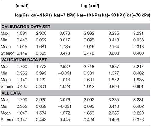
Table 2. Logarithmic saturated hydraulic conductivities (Ks, cm/day) and air permeability (ka, μm2) measured after applying a draining pressure of −4, −7, −10, −30, and −70 kPa for the calibration and validation data sets [minimum values (Min), maximum values (Max), mean values (Mean), and standard deviation (St dev)].
X-ray μCT Images Analysis
The segmentation step, within the image processing scheme, has a great impact on the visible porosity calculated on the X-ray μCT image and on the extracted microscopic measurements (Lamandé et al., 2013; Smet et al., 2017). We, therefore, visually verified the accuracy of the global segmentation on each of the 24 X-ray μCT images by superimposing the grayscale images on the binary images. It appears that the porosity-based global segmentation method did not provide satisfactory results for two soil X-ray μCT images (#6 from the calibration set and #20 from the validation set). Those samples had a large air-filled porosity at h = −1 kPa (Lab_PO); the porosity-based segmentation method increased the threshold (increased μCT_PO) in order to obtain a μCT_PO as close as possible to Lab_PO [resulting threshold of 94 (0–255)]. In addition, the algorithm did not converge for one soil sample (#2), which had a large Lab_PO. Otsu's method was, therefore, applied to those three samples and the global threshold values for samples #2, #6, and #20 were 67, 69, and 69 (0–255), respectively. The threshold values comparisons obtained with the porosity-based method for the other samples supported this processing choice; the averaged threshold value was 63 (± 0.75). Finally, the samples #10, #13, #16 and #17 were segmented using the Otsu's method because their soil water retention curves (SWRC) were not measured. Figure 1 presents a 3D visualization of each soil sample (calibration and validation sets) followed by a 2D vertical slice from the middle of the soil sample. We will refer to this figure within the Results section.
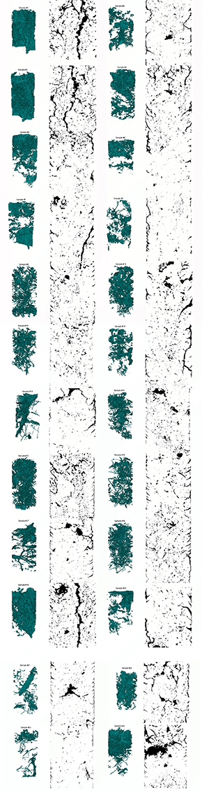
Figure 1. 3D and 2D representations of the 24 studied soil samples.
Microscopic Measurements
Table 3 presents the data ranges, averages and associated standard deviations for all the previously introduced microscopic measurements made on the X-ray μCT soil images (Table 1). The calculated μCT porosities, taking into account pores of at least five voxels, were only slightly higher than those calculated taking into account pores of at least 1,000 voxels. The differences represented ± 90% of the number of pores (the pores having a volume between five and 1,000 voxels happened to be the “small pores” as defined in Table 1). There was no surprise that we observed longer pore networks (L), higher numbers of pore branches (B) and junctions (J) than Katuwal et al. (2015b) or Garbout et al. (2013) who both worked with larger voxel sizes. Consequently to the high number of pores (NP), the observed Euler numbers (ε) were frequently highly positive and the differences between the percentage of isolated pore (IP) and isolated porosity (IPO) was large. Comparisons to others studies are however tricky because the pore network skeleton is highly sensitive to the scanning equipment and procedure, the image processing, the skeletonisation process and the pore identification.
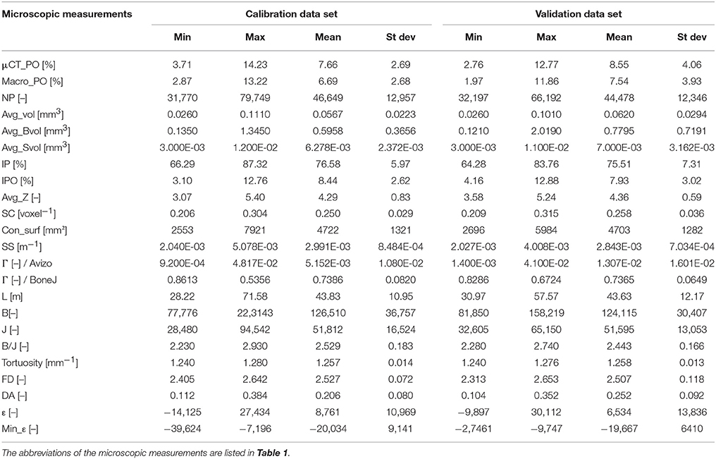
Table 3. Microscopic measurements on μCT X-ray images for the calibration and validation data set [minimum values (Min), maximum values (Max), mean values (Mean), and standard deviation (St dev)].
Table 4 provides the credible (BF > 3) Bayesian correlation coefficients between each of the microscopic measurements. The coefficients were initially calculated for the calibration data and then the validation data were included. In Bayesian statistics, the number of observations does not count for the credibility of a hypothesis, so when a BF was improved with the addition of the validation data, it meant that the correlation was more credible thanks to the observation values. The BF were highlighted with colors according to the classes described in the Materials and Methods section. We did not compute the Bayesian regression equations between microscopic measurements since it was not in the scope of this paper. We did not observe any substantial evidence for the null hypothesis between any of the microscopic measurements.

Table 4. Significant Bayesian correlation coefficients between the microscopic measurements for the calibration data set (Cal. data) or the complete data set (All data).
As Perret et al. (1999) observed, μCT_PO and NP were not correlated; NP cannot be a measure of porosity, but rather expresses a notion of pore density and distribution through the soil sample. The positive correlation between μCT_PO and the fractal dimension (FD) has often been observed in the literature (Rachman et al., 2005; Larsbo et al., 2014) and its dependence on μCT_PO is actually the main drawback of being used as an indicator of pore network heterogeneity and complexity. FD was also correlated to the specific surface area (SS), L, B, J, and NP, which is consistent with studies from Kravchenko et al. (2011) and Anderson (2014). Those five parameters were all highly correlated to each other but selecting one to represent the other could distort the analysis.
The correlation between μCT_PO and average pore volumes (Avg_vol, Avg_Bvol, and Avg_Svol) also made sense since the average pore volumes were not negatively correlated to NP. The average pore volumes were all slightly correlated to Avg_Z; we observed that larger pores tended to be more connected; Avg_Z and Large_PO were also correlated. This is consistent with the results from Luo et al. (2010); Larsbo et al. (2014); Katuwal et al. (2015a,b). Regarding the other connectivity indicators [degree of connectivity (B/J), the Euler number [ε], and the average surface connectivity (SC)], we observed that AvgZ was correlated to B/J but not to ε or to SC while B/J was correlated to ε and not to SC, and SC was correlated to ε. Those connectivity indicators did not carry the exact same information and should, therefore, be used for their potential explanatory power, as pointed out by Renard and Allard (2013) and Katuwal et al. (2015a), Jarvis et al. (2017), and Sandin et al. (2017) have focused on connectivity indicators based on the percolation theory, and they found that four indicators of connectivity were interchangeable and dependent on soil porosity. We calculated the global connectivity (Γ) indicator from the pore size distribution extracted from Avizo and, from the cluster distribution extracted from BoneJ to be comparable to Jarvis et al. (2017) and Sandin et al. (2017). We observed drastically different Γ values from the two methods of computation. As Houston et al. (2017) assessed it, the software, and the decomposition method that goes with it, influence the final pore size distribution. The very low values of Γ from Avizo came from the decomposition of the pore space into a large amount of connected (or not) pores and the resulting smaller (by two orders of magnitude) largest component than the one identified in BoneJ, where cluster of connected pores are quantified. In the following, to be comparable to Sandin et al. (2017), we used the Γ value computed from the BoneJ's cluster size distribution.
Relationships Between the Microscopic and Macroscopic Measurements
Measured, Calculated, and Predicted Soil Water Retention Curves
In the following section, samples #10, #13, #16, and #17 were not included because SWRC were not measured; the calibration data set included 14 samples instead of 18.
Air-filled porosity at h = −1 kPa
In the calibration data set, the relationship between μCT_PO and Lab_PO was neither linear nor credible because of three outliers (#1, #2, #7, Figure 2). As discussed above, samples #2 and #7 were segmented with Otsu's method. In the case of sample #7, Lab_PO was too large for the porosity-based method, introducing unrealistic porosity that would explain the deviations. Lab_PO was calculated by weighing the soil samples after draining. If the pore surfaces were rough or loose, water films could have covered up the pores surface by adsorption and pores could appear smaller than they are. Difference between adsorption and desorption curves, also known as the hysteresis effect, can indeed be substantial close to saturation (McKenzie et al., 2002). A physical explanation for sample #1 could be that it had large pores which drained just before being weighed at saturation. Therefore, the volume of water used to calculate the total laboratory porosity could have been under-evaluated. This is most likely since one gram of water can change the Lab_PO from 8.02 to 14.21%. The 3D visualization of sample #1 shows that a large part of its porosity was connected from top to bottom (Figure 1). The validation data were in agreement with the calibration data except for sample #20, which was segmented with Otsu for the same reasons as sample #7, and sample #22, which showed a behavior similar to sample #1.
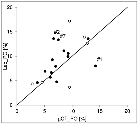
Figure 2. Air-filled porosity measured in the laboratory at a water matric potential of −1 kPa (Lab_PO) vs. the visible porosity measured on X-ray images (μCT_PO) for the calibration data set (black circles) and the validation data set (white circles).
Eventually, the samples that were segmented with the porosity-based method displayed similar Lab_PO and μCT_PO values. Lab_PO was used as a target during the segmentation process. Elliot et al. (2010) also found congruent air-filled porosity values measured by X-ray μCT (voxel size of 453μm3) and by weight determination. The slope of the relationship between Lab_PO and μCT_PO was higher than one and Lab_PO was indeed positively correlated to the difference between Lab_PO and μCT_PO. The applied capillary theory to calculate Lab_PO and μCT_PO simplifies the pore network to capillaries. We, therefore, suggest that the difference between Lab_PO and μCT_PO reflected the systematic error produced by considering pores as capillaries, and increasing the volume of data to which the theory was applied (PO) had increased the error (the difference). The difference between Lab_PO and μCT_PO, whether in absolute value or not, could, however, not be correlated to any microscopic measurements. We presumed that the pore network real connectivity would explain the imperfect applicability of the capillary law. For example, Parvin et al. (2017) reported that the percentage of isolated pores explained the difference in volumetric water content (between laboratory evaporation measurements and X-ray μCT calculation) at a water matric potential ranging from −0.35 to −0.4 kPa by only considering pores larger than 350 μm (pores that should drain at a matric potential of −0.42 kPa from capillary law). The isolated pores were actually connected to others by throats smaller than the voxel size and may not have drained at the required potential calculated from capillary law.
From discrete to continuous data
Beckers et al. (2014a) and Parvin et al. (2017) applied nearly the same methodology to compare predicted SWRC with the bimodal version (Durner, 1994) of the van Genuchten (1980) model. On one hand, they only used macroscopic input data [from pressure plates weighting procedure for Beckers et al. (2014a) and from the evaporation method for Parvin et al. (2017)], and on the other hand, they used those macroscopic data in combination with microscopic data (pore-size distribution extracted from X-ray μCT images) as input. They both found that using the X-ray μCT data allows a better prediction of SWRC close to saturation in terms of RRMSE. We noted, however, that those studies used macroscopic data from one set of soil samples and microscopic data from another set of soil samples. We aimed at validating the results by using the same samples for both types of measurements. To that purpose, capillary theory was applied to the pore-size distribution extracted from the X-ray μCT images and the calculated SWRC were adjusted to the total laboratory porosity. Figure 3 illustrates the SWRC for three samples and shows that for all samples, except #1, the volumetric water content (θ) close to saturation was higher when predicted with the combination of X-ray μCT data and pressure plates data (μCT+PP) than with only the pressure plates data (PP), confirming previous results from Beckers et al. (2014a) to Parvin et al. (2017). We also observed that according to the RRMSE values, prediction with μCT+PP data were better than with only the PP data (Table 5), except for sample #1. Lamandé et al. (2013) also found that X-ray μCT measurements (voxel size of 6003 μm3) allowed a more complete description of the pore space than classical laboratory measurements, and Rab et al. (2014) have concluded that X-ray μCT was likely a better method than laboratory SWRC measurements for determining air-filled macroporosity (pores larger than 300 μm in diameter). The poor performance from sample #1 came from the fact that Lab_PO was lower than μCT_PO, as discussed in Figure 2. Apart from sample #1, the use of microscopic information undeniably improved the prediction of continuous SWRC with the bimodal version (Durner, 1994) of the van Genuchten model (1980).
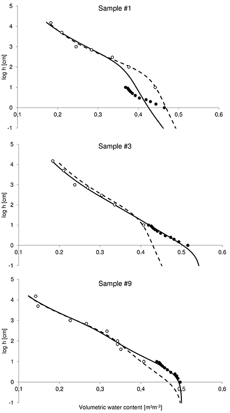
Figure 3. Measured and predicted soil-water retention curves for three samples. Unlike the samples, the SWRC for #1 predicted with the pressure plates data alone (plain line, Pred_PP_DP) performed better than with X-ray μCT data (dotted line, Pred_PP+μCT_DP). Black circles represent the X-ray μCT data and white circles the pressure plate measurements.
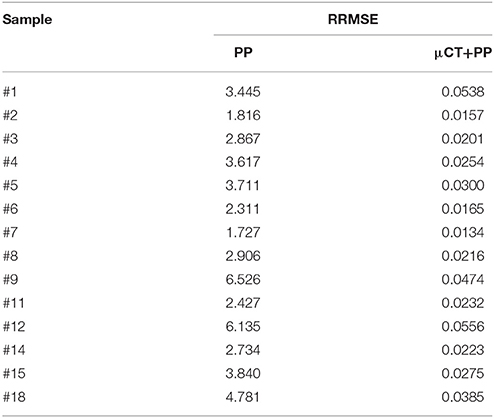
Table 5. Relative root mean squared error (RRMSE, %) for the predicted soil water retention curves with the pressure plates data (PP) or the μCT data plus the pressure plates data (μCT + PP) for the calibration data set samples.
Altogether
The determination of SWRC through pressure plate measurements are likely more representative of the in-situ soil hydrodynamic, but those are not free of artifacts; for example, air entrapment might result in incomplete saturation leading to inaccurate estimation of the air-filled macroporosity. And, although the connectivity of the pore network was not taken into account with the X-ray μCT SWRC calculation, we still observed that the combination of laboratory measurements and X-ray μCT data improved the SRWC prediction close to saturation. The accurate characterization of the air-filled macroporosity is important for the study of microorganism development (e.g., soil fungal growth in Falconer et al., 2012).
Saturated Hydraulic Conductivity and Soil Porous Structure
The saturated hydraulic conductivity was positively correlated to the global connectivity indicator (Γ) computed from the BoneJ cluster size distribution (Figure 4A, ρ = 0.593, BF = 9.5) as observed in Sandin et al. (2017), unlike that study, we did not observe a credible correlation, but a positive trend between μCT_PO and Γ/BoneJ. It is worth noticing again that Sandin et al. (2017) worked with a resolution close to our but with a different textural soil. Pöhlitz et al. (2018) also reported similar trend of Ks and connectivity values (and μCT_PO) between cultural practices. They worked with a voxel size of 603μm3 on different samples for the Ks and microscopic measurements, with although a large number of repetitions. Figure 4A shows the observations of the calibration data (black circles), the observations of the validation data (white circles), the predicted validation points with the 50% quantiles of the regression model (crosses) and the 25 and 75% quantiles of the regression models (dotted lines). The 50% quantiles of the regression models provided a RRMSE of 0.492 for the validation data and the predicted data points were, in most cases, underestimated. The reported regression models that included two explaining variables reported light credible evidence in the cases where Γ was one of the explaining variables. We did not observe relationships between μCT_PO and log(Ks), despite what the literature reported (Kim et al., 2010; Luo et al., 2010; Mossadeghi-Björklund et al., 2016; Naveed et al., 2016). The measured Ks from those studies were, however, higher by several orders of magnitude. We did observe a positive correlation between log(Ks) and FD when the calibration samples were visually separated in two groups according to their Ks value (Figure 4B, black circles). Samples #1, #2, #3, #4, #7, #11, #12, #14, #15, #16, #18 were part of group 1 and samples #5, #6, #8, #9, #10, #13, #17 were part of group 2. No microscopic measurements explained that separation and it was difficult to visually distinguish a pore distribution trend within the pore space (Figure 1). We noticed that some of the less conductive samples presented one or two large macropores (not necessarily vertically oriented nor connected from top to bottom) while some of the more conductive samples had more dispersed pore networks, and we observed a negative trend (not credible) between FD and the degree of anisotropy (DA) for group 2, but not for group 1. This suggested that the porosity arrangement led to the composition of two groups for the relationship between FD and log(Ks). By using the Ks value as a boundary, the validation data were assigned to a group (Figure 4B, white circles). FD measures the ability of the studied object to fill the Euclidian space within which it is integrated and, the larger the FD, the closer to a real fractal the object gets, meaning that its shape is similar at different scales. Although Pachepsky et al. (2000) reported that soils are far from being real fractal, Perret et al. (2003) and Kravchenko et al. (2011) pointed out that FD can be used as a global measure of the pore network complexity. For example, FD was found to vary with depth or soil treatment (Rachman et al., 2005; Udawatta and Anderson, 2008; Kim et al., 2010). Anderson (2014) also observed a positive correlation between log(Ks) and FD. By applying the regression equations, log(Ks) of group 1 equal to log(Ks) of group 2, when FD = 3.03, which was close to the upper limit of the possible FD values of a 3D object. At FD = 3, the object (the porosity) occupies each point of 3D Euclidian space, but that also meant that log(Ks) was limited to 128 cm/day. It is reasonable to ask if more groups would be created with increasing conductivity and if the slopes of the relationships would decrease, or if the solutions of the regression equations would be identical when the fractal dimension equals three, which is the fractal dimension upper limit for an Euclidian 3D object. The global RRMSE was 0.260, which is a rather good performance (Figure 4B, crosses). The 25 and 75% regression model quantiles were highly dispersed (Figure 4B, dotted lines) inducing uncertainty about the regression model.
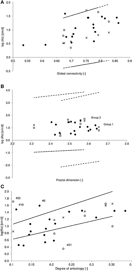
Figure 4. Logarithmic saturated hydraulic conductivity (Ks) vs. (A) global connectivity calculated from the pore size distribution extracted from BoneJ, (B) the fractal dimension measured on X-ray μCT images, and (C) the soil degree of anisotropy measured on X-ray μCT images. Black and white circles represent the observations from the calibration and validation data sets, respectively. Crosses represent predicted validation data points and dotted lines represent the 25 and 75% regression model quantiles.
Anisotropy has been shown to impact soil conductivity (Ursino et al., 2000; Raats et al., 2004; Zhang, 2014). Figure 4C plots log(Ks) as a function of DA (black circles for the observations of the calibration data) and by removing two outliers from the calibration data set (#9 and #10), we obtained a correlation coefficient of 0.74 (BF = 125.3), which presents a convincing link that has, to our knowledge, not been seen before. Such a positive correlation could be interpreted as a consequence of preferential flow through large macropores. For example, Dal Ferro et al. (2013) have found that anisotropy was scale-dependent by showing higher average DA in soil cores (DA of 0.32 and voxel size of 40 μm) than in soil aggregates (DA of 0.14 and voxel size of 6.25 μm), they hypothesized that as a possible consequence of biological and mechanical macropores. This was later confirmed by a second study where they showed that only the macropores in the range of 250–500 μm were correlated to the global DA (Dal Ferro et al., 2014). From the DA calculation decomposition (in the Supplementary Materials section), it was possible, but not straightforwardly, to evaluate the main direction of the anisotropy which could be represented by a small amount of pores in that direction, or as the direction of the preferential orientation of one large pore. Ks was measured along the z-axis (vertically) but the main direction of anisotropy was not systematically in that direction. Therefore, the positive correlation between DA and log(Ks) was not necessarily a result of preferential pore networks paths. Moreover, the directions of the pore connections showed that a majority of the pores junction were horizontal (x- and y-axis). The repartition was practically the same between samples, 60% horizontal and 40% vertical connections. Applying the regression model to the validation data gave consistent results for four samples with a RRMSE for those of 0.414 (Figure 4C, crosses). Sample #21 gave poor results with a predicted log(Ks) of 1.03 cm/day instead of an observed log(Ks) of 0.35 cm/day and a resulting RSE of 3.742. As well, sample #22 gave a RSE of 0.433, its low DA and large log(Ks) made it similar to the two outliers of the calibration data (#9 and #10). The relationship between DA and log(Ks) may not be suitable for highly conductive soil sample presenting isotropic-like porosity distribution (Samples #9, #10, #22, Figure 1). Subjective comparisons between 3D representations and DA need to be made cautiously. We observed that, compared to samples #9, #10, #22, samples #15 and #18 had similar visually homogenous porosity (and equivalent low DA) but with a lower Ks. Samples from group 2 in Figure 4 (#5, #6, #8, #13, #17 and #20, #23, #24) had higher log(Ks) with a more heterogeneous porosity (and higher DA). The narrower distribution of the 25 and 75% regression model quantiles came from the exclusion of two outliers in the model computation.
The prediction of the hydraulic conductivity curve is frequently extracted from the SWRC shape and absolute values of K(h) can be obtained by matching both curves with a specific point, which is often Ks (Vogel and Roth, 1998). Ks is however cumbersome and time-consuming to measure in-situ. We reported here that the porosity arrangement described by the global connectivity, the fractal dimension, and degree of anisotropy had an impact on the soil conductivity, the combination of those indicators provided information that could be used across scales and to eventually better estimate Ks. No other relationships between log(Ks) or Ks and the other microscopic measurements were reported.
Air Permeability Variations Explained by Microscopic Structure
Macroscopic measurements showed, as expected, that the air permeability increased with air-filled porosity. We also observed positive credible Bayesian correlation coefficients between log(ka) measured at various h and microscopic indicators of the porosity (μCT_PO, Large_PO, Avg_vol, Avg_Bvol, and Avg_Svol), although only log(ka,−70 kPa) was positively correlated to μCT_PO (Table 6). Given the X-ray μCT image resolution, μCT_PO should be representative of the air-filled PO measured at h = −1 kPa although th e soil samples were scanned at h = −70 kPa. The choice to scan soil samples at h = −70 kPa was a compromise between the fact that all the potential visible porosity should be air-filled and without cracks due to drying, and this particular correlation suggests that all the potential visible porosity was indeed air-filled. In their study, Katuwal et al. (2015b.) and Naveed et al. (2016) both observed a power-law function between, respectively, ka(−2 kPa) or ka(−3 kPa) and μCT_PO. The μCT_PO calculated on their images is equivalent to the Large_PO on our images as previously stated, and we also reported a correlation between Large_PO and log(ka) (Table 6). Therefore, the difference between μCT_PO and Large_PO might be the part of the PO that should have drained at low negative potential (from the capillary law), but was actually drained at higher negative potential (due to unusable pathways). We refer to Hunt et al. (2013) to name that part of porosity, the inaccessible porosity. This assumption was confirmed by the credible correlations between the inaccessible PO and microscopic parameters which expresses a notion of pore network complexity (B, J, L, NP, SS, IPO, FD). We previously pointed out the drawback that, when calculating SWRC from the X-ray μCT data (namely from the visual pore size distribution), the connectivity was not taken into account. We here confirmed that the pore network connectivity play a role in the desorption process.
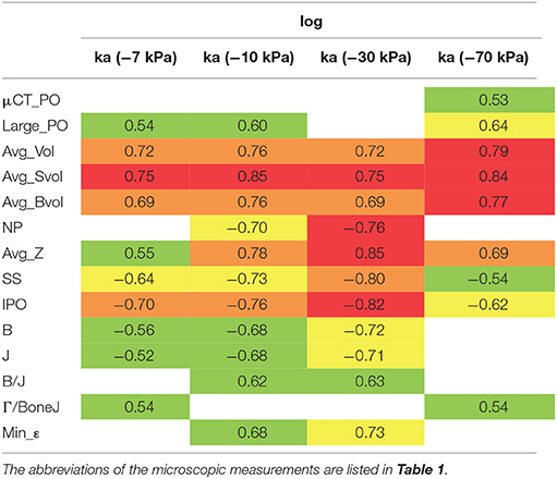
Table 6. Credible Bayesian correlation coefficients between microscopic measurements and logarithmic air permeability (ka) measured at water matric potentials of −70, −30, −10, and −7 kPa for the calibration data set.
Lamandé et al. (2013) found a positive correlation between log(ka,−10 kPa) and NP. We observed negatives correlations (as well as with B, J, and SS). Many pores of our samples were connected to others with connections smaller than the voxel size and were considered isolated (high IP and ε, Table 3). It would make sense, that an increasing volume of small (invisible) connections reduces the airflow through the pore network. The air permeability is also largely dependent on the tortuosity and connectivity of the pore network (Ball and Schjønning, 2002; Moldrup et al., 2003), but to our knowledge, no study has reported these links from μCT measurements. From Table 6, it appears that the air permeability increased with a growing average number of connections (Avg_Z) as well with a growing global connectivity (Γ/BoneJ), but also with Min_ε and B/J. The last two parameters indicate a decreasing connectivity with an increasing value. First, from Table 4, it was observed that B/J increased with decreasing B or decreasing J. That purely algebraic relationship might explain why the air permeability would decrease with decreasing B/J (increasing connectivity). Then, Min_ε was calculated over the largest connected pore component, and, because there are no cavities in real soil pore space (Vogel and Roth, 1998), Min_ε decreased as the number of redundant connections increased. When calculating Avg_Z by class of pore according to their volumes, it appeared that the values of Avg_Z we observed came from a large number of small pores having few connections; the biggest pores had ten times more connections. Avg_Z was correlated to Avg_Z calculated on the pores having a radius between 250 and 375 μm. Therefore, air permeability was correlated to the fact that “medium” size pores had more connections. Moreover, there was a negative trend between log(ka) and Avg_Z calculated on the largest pores which corroborated the positive correlation between ka and Min_ε.
The best regression models calculated on the calibration data (Bayes factor) and applied on the validation data reported that the best explaining variable for all measures of log(ka) (RRMSE) was the average pore volume of the smallest pores (Avg_Svol). That parameter might be seen as a limiting factor, and this suggested that ka was more related to pore size distribution than porosity. Figure 5A displays log(ka, −70 kPa) as a function of Avg_Svol and the distribution of the 25 and 75% regression model quantiles are rather narrow. The RRMSE was 1.256 or 0.0649 when the two worst predicted validation data points were not taken into account. The RRMSE for log(ka, −30 kPa) and log(ka, −10 kPa) were around 0.800 with one bad validation data point, and the RRMSE for log(ka, −7 kPa) was very high (8.154) with three badly predicted data points out of five. The combination of Avg_Svol and average pore volume of all pores (Avg_Vol) performed slightly better in some cases, and slightly worse in others. Figure 5B shows the predicted log(ka) from Avg_Svol vs. the observed log(ka) values. Although the RRMSE were acceptable, the regression model distributions (the error bars represent the 75% regression models quantiles) were high which induce large uncertainty. That combination of two explaining variables was, in all cases, the best regression model of two explaining variables. Other important explaining variables were the average coordination number (Avg_Z), the proportion of isolated porosity (IPO), the average pore volume of the biggest pores (Avg_Bvol) and the combination of μCT_PO and Large_PO.
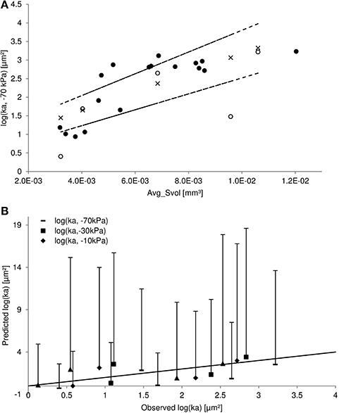
Figure 5. (A) Logarithmic air permeability measured at a water matric potential of −70 kPa (ka) vs. the average pore volume of the smallest pores (Avg_Svol). Black and white circles represent the observations from the calibration and validation data sets, respectively. Crosses represent the predicted validation data points and the dotted lines the 25 and 75% regression model quantiles. (B) The predicted logarithmic air permeability from the average pore volume of the smallest pores vs. the observed logarithmic air permeability. Error bars represent the 75% regression model quantiles.
With soil air diffusivity, soil air permeability is one of the main processes governing the exchange of gases with the atmosphere, including therefore soil aeration. Through our experimentations, we aimed at unraveling the main physical drivers of air fluxes through the soil. We have previously observed that subdividing the pore volume averages into three categories (all of the pores, the biggest, and smallest) was not informative; in this study, we have shown the opposite. Avg_Svol was the average volume of the pores having a volume between 4 × 10⁵ and ± 8 × 107 μm3, in contrast to other cited studies; those pores were visible because of our high resolution (43 μm). Eventually, we suggested that Avg_Svol worked as a limiting factor.
Conclusion
X-ray microtomography, among other visualization techniques, has brought new insight into the study and the understanding of soil function. The challenge, however, is the representativeness of the studied soil samples (Vogel et al., 2010) and, to that purpose, the analysis of the same soil samples at two scales has become more prevalent. The resulting next challenge is the resolution at which the soil samples should be studied. To our knowledge, very few studies dealt with equivalent voxel size (433 μm3) and, we did not find any micro-macro correlations such as the ones we observed.
Starting with the comparison of the calculated visible porosity for all pores and for those of at least 1,000 voxels in volume, it appeared that the difference was rather small but positively correlated to indicators of the pore network complexity. The uncommon relationships we observed might be due to the higher resolution we worked with and the resulting finer details of the pore network structure. For example, the calculated fractal dimension and degree of anisotropy are both global indicators of the pore network complexity and both were positively correlated to the saturated hydraulic conductivity, although with some limitations. The global connectivity showed interesting results although highly dependent on the decomposition software used to extract the pore size distribution. Identifying the key parameters that convey the complexity of the pore network is a motivating goal to reach. Pore network modeling has already proven useful (e.g., Vogel and Roth, 1998, or more recently, Köhne et al., 2011), and those three indicators are values that could be used for the generation of a phenomenological model.
Furthermore, we have reported various positive correlations between the air permeability measured at several water matric potentials and microscopic measurements. The average volume of the smallest pores (as small as ± 4 × 105 μm3) showed the best link with air permeability. Due to our high resolution, we observed a higher number of pores than in other studies and consequently more isolated pores. The Euler number based on the connected space was expected to correlate well with air permeability, but this was not the case. Other measures that provide similar types of information (total pore length, total number of branches, and junctions) proved equally unsatisfactory. In fact, a pertinent link was the positive relationship between the average pore volume of the biggest pores and that of the smallest ones, suggesting dependence between pores of different volumes.
We also reported that the soil water retention curve was better predicted near saturation with the pore size distribution extracted from the X-ray μCT data. Indicators can be derived from the SWRC to characterize soil quality or extrapolate microorganism development (Rabot et al., 2018); its accurate description is therefore a prerequisite. The degree of saturation is also important in the modeling of microbial growth, the dissolution of O2, the soil respiration, the NO and N2O production. These processes are affected by the so-called water filled pore space, by soil oxygen content and by soil temperature, which all vary with the volumetric water content (Smith et al., 2003). Blagodatsky and Smith (2012) concluded that the microbial growth models (and we add to this statement: “among others”) including “an explicit description of microbial growth, i.e., growth rate and efficiency, humidification ratios and their relationship with N availability, need to be coupled with well-developed soil transport models.” The fluid transport predictions for a continuous range of water contents and from discrete measurements are possible through models that are, today, mostly not physically-based. From the pore space structures analyzed, we aimed at contributing to a better understanding of the potential influences of the pore network topology on the physical hydrodynamic properties of soil. Strong unequivocal conclusions could not be drawn because of the limited number of repetitions; image processing and analysis are time-consuming and will be increase with increasing resolution. The comparisons to others studies, as discussed multiple times, depends on many factors and we, therefore, strongly urge the open access to gray scale X-ray μCT images.
Data Availability
Grayscale images and soil physical properties data are available upon request (contact the corresponding author).
Author Contributions
SS conceived and designed the research, acquired and analyzed the X-ray images, analyzed and interpreted the data, and wrote the manuscript. EB provided the general X-ray μCT images processing scheme. EP implemented the 3D morphological quantification's code in Avizo. SS, EB, EP, AL, and AD edited the manuscript.
Funding
This work was funded through a Ph.D. grant awarded to SS (FRIA, FNRS, Brussels, Belgium) and a FNRS grant awarded to EP (R.FNRS.3363–T.1094.14).
Conflict of Interest Statement
The authors declare that the research was conducted in the absence of any commercial or financial relationships that could be construed as a potential conflict of interest.
Acknowledgments
The authors acknowledge the support of the National Fund for Scientific Research (Brussels, Belgium). We also thank Professor Yves Brostaux for his advices on statistical analysis and EP for its availability and expertise. The reviewers are also thanked for their constructive comments.
Supplementary Material
The Supplementary Material for this article can be found online at: https://www.frontiersin.org/articles/10.3389/fenvs.2018.00020/full#supplementary-material
Abbreviations
h, water matric potential; θ, water content; SWRC, soil water retention curve; Ks, saturated hydraulic conductivity; ka, air permeability; LabPO, laboratory measured air-filled porosity at a water matrix potential of 1 kPa; BF, Bayes factor. The rest of the uncommon abbreviations are defined in Table 1.
References
Anderson, S. H. (2014). Tomography-measured macropore parameters to estimate hydraulic properties of porous media. Procedia Comput. Sci. 36, 649–654. doi: 10.1016/j.procs.2014.09.069
Ball, B. C., and Schjønning, P. (2002). “Air permeability,” in Methods of Soil Analysis, Part 1, ed. J. H. Dane and G. C Topp (Madison, WI: Soil Science Society of America), 1141–1158.
Baveye, P. C., and Laba, M. (2015). Moving away from the geostatistical lamppost: why, where, and how does the spatial heterogeneity of soils matter? Ecol. Model. 298, 24–38. doi: 10.1016/j.ecolmodel.2014.03.018
Baveye, P. C., Pot, V., and Garnier, P. (2017). Accounting for sub-resolution pores in models of water and solute transport in soils based on computed tomography images: are we there yet? J. Hydrol. 555, 253–256. doi: 10.1016/j.jhydrol.2017.10.021
Beckers, E., Plougonven, E., Gigot, N., Léonard, A., Roisin, C., Brostaux, Y., et al. (2014a). Coupling X-ray microtomography and macroscopic soil measurements: a method to enhance near saturation functions? Hydrol. Earth Syst. Sci. 18, 1805–1817. doi: 10.5194/hess-18-1805-2014
Beckers, E., Plougonven, E., Roisin, C., Hapca, S., Léonard, A., and Degr,é, A. (2014b). X-ray microtomography: a porosity-based thresholding method to improve soil pore network characteristization? Geoderma 219–220, 145–154. doi: 10.1016/j.geoderma.2014.01.004
Blagodatsky, S., and Smith, P. (2012). Soil physics meets soil biology: towards better mechanistic prediction of greenhouse gas emissions from soil. Soil Biol. Biochem. 47, 78–92. doi: 10.1016/j.soilbio.2011.12.015
Corey, A. T. (1986). “Air permeability,” in Methods of Soil Analysis. Part I. 2nd Edn, ed A. Klute (Madison, WI: Agronomy Monograph 9, American Society of Agronomy, Inc.; Soil Science Society of America, Inc.,), 1121–1136.
Cousin, I., Levitz, P., and Bruand, A. (1996). Three-dimensional analysis of a loamy-clay soil using pore and solid chord distributions. Eur. J. Soil Sci. 47, 439–452. doi: 10.1111/j.1365-2389.1996.tb01844.x
Crestana, S., Mascarenhas, S., and Pozzi-Mucelli, R. S. (1985). Static and dynamic three-dimensional studies of water in soil using computed tomographic scanning. Soil Sci. 140, 326–332. doi: 10.1097/00010694-198511000-00002
Dal Ferro, N., Charrier, P., and Morari, F. (2013). Dual-scale micro-CT assessment of soil structure in a long-term fertilization experiment. Geoderma 204–205, 84–93. doi: 10.1016/j.geoderma.2013.04.012
Dal Ferro, N., Sartori, L., Simonetti, G., Berti, A., and Morari, F. (2014). Soil macro- and microstructure as affected by different tillage systems and their effects on maize root growth. Soil Til. Res. 140, 55–65. doi: 10.1016/j.still.2014.02.003
Dal Ferro, N., Strozzi, A. G., Duwig, C., Delmas, P., Charrier, P., and Morari, F. (2015). Application of smoothed particle hydrodynamics (SPH) and pore morphologic model to predict saturated water conductivity from X-ray CT imaging in a silty loam Cambisol. Geoderma 255–256, 27–34. doi: 10.1016/j.geoderma.2015.04.019
DIN ISO 11274 (2012). Soil Quality–Determination of the Water Retention Characteristics–Laboratory Methods (ISO 11274:1998 + Cor. 1:2009) English Translation of DIN ISO 11274, 2012-04. Deutsches Institut für Normung, Berlin.
Doube, M., Klosowski, M. M., Arganda-Carreras, I., et al. (2010). Bone-J: free and extensible bone image analysis in ImageJ. Bone 47, 1076–1079. doi: 10.1016/j.bone.2010.08.023
Durner, W. (1994). Hydraulic conductivity estimation for soils with heterogeneous pore structure. Water Resour. Res. 30, 211–223. doi: 10.1029/93WR02676
Elliot, T. R., Reynolds, W. D., and Heck, R. J. (2010). Use of existing pore models and X-ray computed tomography to predict saturated soil hydraulic conductivity. Geoderma 156, 133–142. doi: 10.1016/j.geoderma.2010.02.010
Falconer, E. R., Houston, A. N., Otten, W., and Baveye, P. C. (2012). Emergent behavior of soil fungal dynamics: influence of soil architecture and water distribution. Soil Sci. 177, 111–119. doi: 10.1097/SS.0b013e318241133a
Garbout, A., Munkholm, L. J., and Hansen, S. B. (2013). Tillage effects on topsoil structural quality assessed using X-ray CT, soil cores and visual soil evaluation. Soil Til. Res. 128, 104–109. doi: 10.1016/j.still.2012.11.003
Grevers, M. C. J., De Jong, E., and St Arnaud, R. J. (1989). The characterization of soil macroporosity with CT scanning. Can. J. Soil Sci. 69, 629–637. doi: 10.4141/cjss89-062
Gutiérrez Castorena, E. V., Gutiérrez Castorena, M. D. C., Vargas, T. G., Bontemps, L. C., Martinez, J. D., Mendez, E. S., et al. (2016). Micromapping of microbial hotspots and biofilms from different crops using image mosaics of soil thin sections. Geoderma 279, 11–21. doi: 10.1016/j.geoderma.2016.05.017
Harrigan, T. P., and Mann, R. W. (1984). Characterization of microstructural anisotropy in orthotropic materials using a 2nd rank tensor. J. Mater. Sci. 19, 761–767. doi: 10.1007/BF00540446
Houston, A. N., Otten, W., Falconer, R., Monga, O., Baveye, P. C., and Hapca, S. M. (2017). Quantification of the pore size distribution of soils: assessment of existing software using tomographic and synthetic 3D images. Geoderma 299, 73–82. doi: 10.1016/j.geoderma.2017.03.025
Houston, A. N., Schmidt, S., Tarquis, A. M., Otten, W., Baveye, P. C., and Hapca, S. (2013). Effect of scanning and image reconstruction settings in X-ray computed microtomography on quality and segmentation of 3D soil images. Geoderma 207–208, 154–165. doi: 10.1016/j.geoderma.2013.05.017
Hunt, A. G., Ewing, R. P., and Horton, R. (2013). What's wrong with soil physics? Soil Sci. Soc. Am. J. 77, 1877–1887. doi: 10.2136/sssaj2013.01.0020
Jarvis, N., Larsbo, M., and Koestel, J. (2017). Connectivity and percolation of structural pore networks in a cultivated silt loam soil quantified by X-ray tomography. Geoderma 287, 71–79. doi: 10.1016/j.geoderma.2016.06.026
Katuwal, S., Moldrup, P., Lamandé, M., Tuller, M., and de Jonge, L. W. (2015a). Effect of CT number derived matrix density on preferential flow and transport in a macroporous agricultural soil. Vadose Zone J. 14, 1–13. doi: 10.2136/v15.01.0002
Katuwal, S., Norgaard, T., Moldrup, P., Lamandé, M., Wildenschild, D., and de Jonge, L. W. (2015b). Linking air and water transport in intact soils to macropore characteristics inferred from X-ray computed tomography. Geoderma 237–238, 9–20. doi: 10.1016/j.geoderma.2014.08.006
Kim, H., Anderson, S. H., Motavalli, P. P., and Gantzer, C. J. (2010). Compaction effects on soil macropore geometry and related parameters for an arable field. Geoderma 160, 244–251. doi: 10.1016/j.geoderma.2010.09.030
Koestel, J., and Larsbo, M. (2014). Imaging and quantification of preferential solute transport in soil macropores. Water Resour. Res. 50, 4357–4378. doi: 10.1002/2014WR015351
Köhne, J. M., Schlüter, S., and Vogel, H.-J. (2011). Predicting solute transport in structured soil using pore network models. Vadose Zone J. 10, 1082–1096. doi: 10.2136/vzj2010.0158
Kravchenko, A. N., and Guber, A. K. (2017). Soil pores and their contributions to soil carbon processes. Geoderma 287, 31–39. doi: 10.1016/j.geoderma.2016.06.027
Kravchenko, A. N., Wang, A. N. W., Smucker, A. J. M., and Rivers, M. L. (2011). Long-term differences in tillage and land use affect intra-aggregate pore heterogeneity. Soil Sci. Soc. Am. J. 75, 1658–1666. doi: 10.2136/sssaj2011.0096
Lamandé, M., Wildenschild, D., Berisso, F. E., Garbout, A., Marsh, M., Moldrup, P., et al. (2013). X-ray CT and laboratory measurements on glacial till subsoil cores: assessment of inherent and compaction-affected soil structure characteristics. Soil Sci. 178, 359–368. doi: 10.1097/SS.0b013e3182a79e1a
Larsbo, M., Koestel, J., and Jarvis, N. (2014). Relations between macropore network characteristics and the degree of preferential solute transport. Hydrol. Earth Syst. Sci. 18, 5255–5269. doi: 10.5194/hess-18-5255-2014
Legland, D., Arganda-Carreras, I., and Andrey, P. (2016). MorphoLibJ: integrated library and plugins for mathematical morpholofy with ImageJ. Bioinformatics 32, 3532–3534. doi: 10.1093/bioinformatics/btw413
Liang, F., Paulo, R., Molina, G., Clyde, M. A., and Berger, J. O. (2008). Mixtures of g-priors for Bayesian variable selection. J. Am. Stat. Assoc. 103, 410–423. doi: 10.1198/016214507000001337
Loll, P., Moldrup, P., Schjønning, P., and Riley, H. (1999). Predicting saturated hydraulic conductivity from air permeability: application in stochastic water infiltration modeling. Water Resour. Res. 35, 2387–2400. doi: 10.1029/1999WR900137
Luo, L., Lin, H., and Halleck, P. (2008). Quantifying soil structure and preferential flow in intact soil using X-ray computed tomography. Soil Sci. Soc. Am. J. 72, 1058–1069. doi: 10.2136/sssaj2007.0179
Luo, L., Lin, H., and Schmidt, J. (2010). Quantitative relationships between soil macropore characteristics and preferential flow and transport. Soil Sci. Soc. Am. J. 74, 1929–1937. doi: 10.2136/sssaj2010.0062
Marin, J.-M., and Robert, C. P. (2007). Bayesian Core. A Pratical Approach to Computational Bayesian Statistics. New York, NY: Springer.
McKenzie, N., Coughlan, K., and Cresswell, H. (2002). Soil Physical Measurement and Interpretation for Land Evaluation. Collingwood: CSIRO Publishing.
Moldrup, P., Yoshikawa, S., Olesen, T., Komatsu, T., and Rolston, D. E. (2003). Air permeability in undisturbed volcanic ash soils: predictive model test and soil structure finderprint. Soil Sci. Soc. Am. J. 67, 32–40. doi: 10.2136/sssaj2003.3200
Monga, O., Garnier, P., Pot, V., Coucheney, E., Nunan, N., Otten, W., et al. (2014). Simulating microbial degradation of organic matter in a simple porous system using the 3-D diffusion-based model MOSAIC. Biogeosciences 11, 2201–2209. doi: 10.5194/bg-11-2201-2014
Morey, R. D., and Rouder, J. N. (2015). BayesFactor: Computation of Bayes Factors for Common Designs. R package version 0.9.12-2. Available online at: https://CRAN.R-project.org/package=BayesFactor
Mossadeghi-Björklund, M., Arvidsson, J., Keller, T., Koestel, J., Lamandé, M., Larsbo, M., et al. (2016). Effects of subsoil compaction on hydraulic properties and preferential flow in a Swedish clay soil. Soil Til. Res. 156, 91–98. doi: 10.1016/j.still.2015.09.013
Naveed, M., Moldrup, P., Arthur, E., Wildenschild, D., Eden, M., Lamandé, M., et al. (2012). Revealing soil structure and functional macroporosity along a clay gradient using X-ray computed tomography. Soil Sci. Soc. Am. J. 77, 403–411. doi: 10.2136/sssaj2012.0134
Naveed, M., Moldrup, P., Schaap, M. G., Tuller, M., Kulkarni, R., Vogel, H.-J., et al. (2016). Prediction of biopore- and matrix-dominated flow from X-ray CT-derived macropore networkds characteristics. Hydrol. Earth. Syst. Sci. 20, 4017–4030. doi: 10.5194/hess-20-4017-2016
Nuijten, M. B., Wetzels, R., Matzke, D., Dolan, C. V., and Wagenmakers, E.-J. (2015). BayesMed: Default Bayesian Hypothesis Tests for Correlation, Partial Correlation, and Mediation. R package version 1.0.1. Available online at: http://CRAN.R-project.org/package=BayesMed
Olson, M. S., Tillman, F. D. Jr., Choi, J.-W., and Smith, J. A. (2001). Comparison of three techniques to measure unsaturated-zone air permeability at Picatinny Arsenal, N. J. J. Contam. Hydrol. 53, 1–19. doi: 10.1016/S0169-7722(01)00135-8
Or, D., Smets, B. F., Wraith, J. M., Deschene, A., and Friedman, S. P. (2007). Physical constraint affecting bacterial habittats and activity in unsaturated porous media – a review. Adv. Wat. Res. 30, 1505–1527. doi: 10.1016/j.advwatres.2006.05.025
Otsu, N. (1979). A threshold selection method from gray-level histograms. IEEE Trans. Syst. Man Cybern. 9, 62–66. doi: 10.1109/TSMC.1979.4310076
Pachepsky, Y. A., Giménez, D., Crawford, J. W., and Rawls, W. J. (2000). “Conventional and fractal geometry in soil science,” in Developments in Soil Science, eds Y. A. Pachepsky, J. W. Crawford and W. J. Rawls (Elsevier), 7–18.
Paradelo, M., Katuwal, S., Moldrup, P., Norgaard, T., Herath, L., and de Jonge, L. W. (2016). X-ray CT-derived characteristics explain varying air, water, and solute transport properties across a loamy field. Vadose Zone J. 192, 194–202. doi: 10.2136/vzj2015.07.0104
Parvin, N., Beckers, E., Plougonven, E., Léonard, A., and Degré, A. (2017). Dynamic of soil drying close to saturation: what can we learn from a comparison between X-ray computed microtomography and the evaporation method? Geoderma 302, 66–75. doi: 10.1016/j.geoderma.2017.04.027
Peng, S., Marone, F., and Dultz, S. (2014). Resolution effect in X-ray microcomputed tomography imaging and small pore's contribution to permeability for a Berea sandstone. J. Hydrol. 510, 403–411. doi: 10.1016/j.jhydrol.2013.12.028
Perret, J. S., Prasher, S. O., and Kacimov, A. R. (2003). Mass fractal dimension of soil macropores using computed tomography: from the box-counting to the cube-counting algorithm. Eur. J. Soil Sci. 54, 569–579. doi: 10.1046/j.1365-2389.2003.00546.x
Perret, J. S., Prasher, S. O., Kantzas, A., and Langford, C. (1999). Three-dimensional quantification of macropore networks in undisturbed soil cores. Soil Sci. Soc. Am. J. 63, 1530–1543. doi: 10.2136/sssaj1999.6361530x
Plougonven, E. (2009). Link between the Microstructure of Porous Materials and their Permeability. Ph.D. thesis, Université Sciences et Technologies, Bordeaux.
Pöhlitz, J., Rücknagel, J., Koblenz, B., Schlüter, S., Vogel, H.-J., and Christen, O. (2018). Computed tomography and soil physical measurements of compaction behavior under strip tillage, mulch tillage and no tillage. Soil Til. Res. 175, 205–2016. doi: 10.1016/j.still.2017.09.007
Pot, V., Peth, S., Monga, O., Vogel, L. E., Genty, A., Garnier, P., et al. (2015). Three-dimensional distribution of water and air in soil pores: comparison of two-phase two-relaxation-times lattice-Boltzmann and morphological model outputs with synchrotron X-ray computed tomography data. Adv. Water Res. 87, 87–102. doi: 10.1016/j.advwatres.2015.08.006
Raats, P. A. C., Zhang, Z. F., Ward, A. L., and Gee, G. W. (2004). The relative connectivity-tortuosity tensor for conduction of water in anisotropic unsaturated soils. Vadose Zone J. 3, 1471–1478. doi: 10.2136/vzj2004.1471
Rab, M. A., Haling, R. E., Aarons, S. R., Hannah, M., Young, I. M., and Gibson, D. (2014). Evaluation of X-ray computed tomography for quantifying macroporosity of loamy pasture soils. Geoderma 213, 460–470 doi: 10.1016/j.geoderma.2013.08.037
Rabot, E., Wiesmeier, M., Schlüter, S., and Vogel, H.-J. (2018). Soil structure as an indicator of soil functions: a review. Geoderma 314, 122–137. doi: 10.1016/j.geoderma.2017.11.009
Rachman, A., Anderson, S. H., and Gantzer, C. J. (2005). Computed-Tomographic measurement of soil macroporosity parameters as affected by stiff-stemmed grass hedges. Soil Sci. Soc. Am. J. 69, 1609–1616. doi: 10.2136/sssaj2004.0312
R Core Team (2015). R: A Language and Environment for Statistical Computing. Vienna: R Foundation for Statistical Computing.
Renard, P., and Allard, D. (2013). Connectivity metrics for subsurface flow and transport. Adv. Wat. Res. 51, 168–196. doi: 10.1016/j.advwatres.2011.12.001
Richards, L. A. (1948). Porous plate apparatus for measuring moisture retention and transmission by soils. Soil Sci. 66, 105–110. doi: 10.1097/00010694-194808000-00003
Roose, T., Keyes, S. D., Daly, K. R., Carminati, A., Otten, W., Vetterlein, D., et al. (2016). Challenges in imaging and predictive modeling of rhizosphere processes. Plant Soil. 407, 9–38. doi: 10.1007/s11104-016-2872-7
Rowell, D. L. (1994). Soil Science: Methods and Application. Harlow, UK: Longman Group Limited, Longman Scientific & Technical.
Sammartino, S., Lissy, A.-S., Bogner, C., Van Den Bogeart, R., Capowiez, Y., et al. (2015). Identifying the functional macropore network related to preferential flow in structured soils. Vadose Zone J. 14, 1–16. doi: 10.2136/vzj2015.05.0070
Sandin, M., Koestel, J., Jarvis, N., and Larsbo, M. (2017). Post-tillage evolution of structural pore space and saturated and near-saturated hydraulic conductivity in a clay loam soil. Soil Til. Res. 165, 161–168. doi: 10.1016/j.still.2016.08.004
Schaap, M. G., Porter, M. L., Christensen, B. S. B., and Wildenschild, D. (2007). Comparison of pressure-saturation characteristics derived from computed tomography and lattice Boltzmann simulations. Water Resour. Res. 43:W12S06. doi: 10.1029/2006WR005730
Schmid, B., Schindelin, J., Cardona, A., Longhair, M., and Heisenberg, M. (2010). A high-level 3D visualization API for Java and ImageJ. BMC Bioinformatics 11:274. doi: 10.1186/1471-2105-11-274
Schneider, C. A., Rasband, W. S., and Eliceiri, K. W. (2012). NIH Image to ImageJ: 25 years of image analysis. Nat. Methods 9, 671–675. doi: 10.1038/nmeth.2089
Shah, S. M., Gray, F., Crawshaw, J. P., and Boek, E. S. (2016). Micro-computed tomography pore-scale study of flow in porous media: effect of voxel resolution. Adv. Wat. Res. 95, 276–287. doi: 10.1016/j.advwatres.2015.07.012
Smet, S., Plougonven, E., Léonard, A., Degré, A., and Beckers, E. (2017). X-ray Micro-CT: how soil pore space description can be altered by image processing. Vadose Zone J. 17:160049. doi: 10.2136/vzj2016.06.0049
Smith, K. A., Ball, T., Conen, F., Dobbie, K. E., Massheder, J., and Rey, A. (2003). Exchange of greenhouse gases between soil and atmosphere: interactions of soil physical factors and biological processes. Eur. J. Soil Sci. 54, 779–791. doi: 10.1046/j.1351-0754.2003.0567.x
Taina, I. A., Heck, R. J., and Elliot, T. R. (2008). Application of X-ray computed tomography to soil science: a literature review. Can. J. Soil Sci. 88, 1–20. doi: 10.4141/CJSS06027
Tarplee, M., and Corps, N. (2008). Skyscan 1072 desktop X-ray microtomograph. sample scanning reconstruction, analysis and visualisation (2D and 3D) Protocols. Guidelines, notes, selected references and F.A.Qs.
Tracy, S. R., Daly, K. R., Sturrock, C. J., Crout, N. M. J., Mooney, S. J., and Roose, T. (2015). Three-dimensional quantification of soil hydraulic properties using X-ray computed tomography and image-based modeling. Water Resour. Res. 51, 1006–1022. doi: 10.1002/2014WR016020
Udawatta, R. P., and Anderson, S. H. (2008). CT-measured pore characteristics of surface and subsurface soils influenced by agroforestry and grass buffers. Geoderma 145, 381–389. doi: 10.1016/j.geoderma.2008.04.004
Ursino, N., Roth, K., Gimmi, T., and Flühler, H. (2000). Upscaling of anisotropy in unsaturated Miller-similar porous media. Water Resour. Res. 36, 421–430. doi: 10.1029/1999WR900320
van Genuchten, M. T. (1980). A closed-form equation for prediction the hydraulic conductivity of unsaturated soils. Soil Sci. Soc. Am. J. 44, 892–898. doi: 10.2136/sssaj1980.03615995004400050002x
Vogel, H.-J. (2000). A numerical experiment on pore size, pore connectivity, water retention, permeability, and solute transport using network models. Eur. J. Soil Sci. 51, 99–105. doi: 10.1046/j.1365-2389.2000.00275.x
Vogel, H.-J., and Roth, K. (1998). A new approach for determining effective soil hydraulic functions. Eur. J. Soil Sci. 49, 547–556. doi: 10.1046/j.1365-2389.1998.4940547.x
Vogel, H.-J., Tölke, J., Schulz, V. P., Krafczyk, M., and Roth, K. (2005). Comparison of a lattice-boltzmann model, a full-morphology model, and a pore network model for determining capillary pressure–saturation relationships. Vadose Zone J. 4, 380–388. doi: 10.2136/vzj2004.0114
Vogel, L. E., Makowski, D., Garnier, P., Vieublé-Gonod, L., Coquet, Y., Raynaud, X., et al. (2015). Modeling the effect of soil meso- and macropores topology on the biodegradation of a soluble carbon substrate. Adv. Water Res. 83, 123–136. doi: 10.1016/j.advwatres.2015.05.020
Vogel, H.-J., Weller, U., and Schlüter, S. (2010). Quantification of soil structure based on Minkowski functions. Comput. Geosci. 36, 1236–1245. doi: 10.1016/j.cageo.2010.03.007
Wagenmakers, E.-J., Verhagen, J., and Ly, A. (2016). How to quantify the evidence for the absence of correlation. Behav. Res. 48, 412–426. doi: 10.3758/s13428-015-0593-0
Wetzels, R., and Wagenmakers, E.-J. (2012). A default Bayesian hypothesis test for correlations and partial correlations. Psychon. Bull. Rev. 19, 1057–1064. doi: 10.3758/s13423-012-0295-x
Wildenschild, D., and Sheppard, A. P. (2013). X-ray imaging and analysis techniques for quantifying pore-scale structure and processes in subsurface porous medium systems. Adv. Water Res. 51, 217–246. doi: 10.1016/j.advwatres.2012.07.018
Young, I. M., Blanchart, E., Chenu, C., Dangerfield, M., Fragoso, C., Grimaldi, M., et al. (1998). The interaction of soil biota and soil structure under global change. Global Change Biol. 4, 703–712. doi: 10.1046/j.1365-2486.1998.00194.x
Keywords: soil, X-ray micro-computed tomography, saturated hydraulic conductivity, soil water retention curve, air permeability, Bayesian statistics
Citation: Smet S, Beckers E, Plougonven E, Léonard A and Degré A (2018) Can The Pore Scale Geometry Explain Soil Sample Scale Hydrodynamic Properties? Front. Environ. Sci. 6:20. doi: 10.3389/fenvs.2018.00020
Received: 30 January 2018; Accepted: 05 April 2018;
Published: 23 April 2018.
Edited by:
Philippe C. Baveye, AgroParisTech Institut des Sciences et Industries du Vivant et de L'environnement, FranceReviewed by:
Steffen Schlüter, Helmholtz-Zentrum für Umweltforschung (UFZ), GermanyNicholas Jarvis, Swedish University of Agricultural Sciences, Sweden
Copyright © 2018 Smet, Beckers, Plougonven, Léonard and Degré. This is an open-access article distributed under the terms of the Creative Commons Attribution License (CC BY). The use, distribution or reproduction in other forums is permitted, provided the original author(s) and the copyright owner are credited and that the original publication in this journal is cited, in accordance with accepted academic practice. No use, distribution or reproduction is permitted which does not comply with these terms.
*Correspondence: Sarah Smet, sarah.smet@uliege.be