Estimating Canopy Parameters Based on the Stem Position in Apple Trees Using a 2D LiDAR

Abstract

Data of canopy morphology are crucial for cultivation tasks within orchards. In this study, a 2D light detection and range (LiDAR) laser scanner system was mounted on a tractor, tested on a box with known dimensions (1.81 m × 0.6 m × 0.6 m), and applied in an apple orchard to obtain the 3D structural parameters of the trees (n = 224). The analysis of a metal box which considered the height of four sides resulted in a mean absolute error (MAE) of 8.18 mm with a bias (MBE) of 2.75 mm, representing a root mean square error (RMSE) of 1.63% due to gaps in the point cloud and increased incident angle with enhanced distance between laser aperture and the object. A methodology based on a bivariate point density histogram is proposed to estimate the stem position of each tree. The cylindrical boundary was projected around the estimated stem positions to segment each individual tree. Subsequently, height, stem diameter, and volume of the segmented tree point clouds were estimated and compared with manual measurements. The estimated stem position of each tree was defined using a real time kinematic global navigation satellite system, (RTK-GNSS) resulting in an MAE and MBE of 33.7 mm and 36.5 mm, respectively. The coefficient of determination (R²) considering manual measurements and estimated data from the segmented point clouds appeared high with, respectively, R² and RMSE of 0.87 and 5.71% for height, 0.88 and 2.23% for stem diameter, as well as 0.77 and 4.64% for canopy volume. Since a certain error for the height and volume measured manually can be assumed, the LiDAR approach provides an alternative to manual readings with the advantage of getting tree individual data of the entire orchard.

1. Introduction

Information on geometrical and structural characteristics of fruit trees provides decisive knowledge for management within the orchard. The geometrical (height, width, and volume) and the structural (the leaf area, leaf density, trunk, and angle of branches) variables affect economically relevant parameters, such as the tree water needs [1,2,3], fruit quality [4,5], and the yield [6]. The manual measurement of tree variables is usually inaccurate and time-consuming. Thus, the performance of measurements in orchards for management purposes lack feasibility at the present state of the art.

Among other instrumental methods for this purpose, the light detection and range (LiDAR) laser scanning seems to be the most adequate for the nondestructive monitoring of geometrical and structural parameters in fruit trees [7], because it (i) operates with an active light source that avoids perturbing effects of varying lighting conditions, (ii) enables higher frequencies than those provided by manual measurements, and (iii) enables us to measure from a distance in multiple directions using one single sensor. A laser diode emits photons with low dispersion, which are reflected back to the photodiode of the scanner when hiting an object. The time between the emission and the reflection of the beam is proportional to the distance among the scanner and the objects, considering the constant of light velocity and sensor response functions. A motor sweeps the laser beam in a plane, describing the shape of objects in two dimensions (2D).

However, in agriculture, the 2D LiDAR has been frequently mounted on a tractor together with a high precision geographical position system to obtain three dimensional (3D) data of trees [8,9,10]. Several studies used this configuration to estimate the structural parameters of fruit trees by segmenting the row point cloud into slices of a constant distance [4,9,10,11]. The canopy volume of the tree row revealed a high correlation coefficient (r) with the manual reference measurement (r = 0.906, p < 0.0001) in olive orchards using the aforementioned method [10]. In another study, Sanz and co-workers [12] used the volume of a tree row to obtain the leaf area, describing a high coefficient of determination (R²) in different chronological stages with a logarithmic model in apple trees (R² = 0.85), pear trees (R² = 0.84), and vines (R² = 0.86). Moreover, several methodologies have been developed for volume extraction such as the convex-hull clustering or voxel grid in vines, olives, and apples [2,13,14], while the alpha shape clustering was applied in citrus [15]. Jimenez-Berni and co-authors [16] described the analysis of plant height in wheat with a strong correlation (R² = 0.99), when using a 2D LiDAR. Furthermore, the leaf area index can be estimated by utilizing the cross-sectional area in vines and apple trees [5,13,17]. Similarly, correlations of pruning weight and vine wood volume resulted in high coefficients of determination with LiDAR measurements (R² = 0.91; R² = 0.76, respectively) [18].

The point cloud clustering for separating single plants was already performed with fixed distances between the trees [13], the convex-hull approach [14], and hidden semi-Markov model [19,20]. Reiser et al. [20] determined the stem position of maize plants using an initial plant and the fixed plant spacing to search iteratively for the best clusters. The height profile of the clustered maize plants estimated, revealed a 33 mm deviation from the manual reference readings. Garrido et al. [21] used a LiDAR and a light curtain to detect stem positions of almond trees, with a detection accuracy of 99.5%. The position of the detected stems was obtained with the help of an optical wheel odometer that separated plants with no overlapping leaves. Zhang and Grift [22] proposed a LiDAR height measurement system for Miscanthus giganteus based on stem density. In static mode, the sensor kept stationary and an average error of 5.08% was achieved, while in the dynamic mode, the sensor was driven past a field edge, which resulted in an average error of 3.8%. In another study, the 2D histogram was used to obtain the height profile in 3D point clouds of cotton plants, resulting in a strong correlation (R² = 0.98) with manual measurements [23]. Moreover, the stem position in maize plants was determined based on bivariate point density histograms in order to find the regional maxima [24]. Thus, single plant segmentation was carried out by projecting a spatial cylindrical boundary around the estimated stem positions of plant point clouds. The maize stem positions were estimated with mean error and standard deviation of 24 mm and 14 mm difference from the actual stem position, respectively. For the overall plant height profile, an error of 8.7 mm was found while considering the manually obtained height.

The overall aim of this research was to propose a methodology for determining the stem position of apple trees by means of a 2D LiDAR system as a basis for separation of trees in commercial orchards. The specific objectives were to test the measuring uncertainty of the LiDAR system, when analyzing a box with known dimensions in the field and real-world trees. The analysis of tree point clouds was evaluated by estimating the height, the stem and the canopy volume of singularized trees. The innovation of this study is the application of the proposed methodology in fruit trees, providing an accurate and precise estimation of geometric variables of apple trees within the orchard.

2. Material and Methods

2.1. Field Experiments

The experiment was conducted in the Leibniz Institute of Agricultural Engineering and Bioeconomy (ATB) experimental station located in Marquardt, Germany (Latitude: 52.466274° N, Longitude: 12.57291° E) in early July of 2018. The orchard was located on 8% slope with southeast orientation. The orchard was planted with trees of Malus × domestica Borkh. ‘Gala’ and ‘JonaPrince’, and pollinator trees ‘Red Idared’ each on M9 rootstock (n = 224) with 0.95 m distance between trees, trained as slender spindle, which form the majority of apple trees in world-wide production, with an average tree height of 2.5 m. No pollinator trees were excluded from the study, since they appeared to have a similar tree architecture to the aforementioned tree types, and were also trained as slender spindles. Trees were supported by means of horizontally parallel wires. Data acquisition was performed at the end of fruit cell division, after a native fruit drop in June. The tractor that was carrying the sensor-frame was driven along each side of the two rows measured, with an average speed of 0.13 m s⁻¹.

The stem position of each tree (n = 224) was defined with a real time kinematic global navigation satellite system (RTK-GNSS), while in parallel a wooden meter was used to estimate the tree height manually (H_manual). The average width of each tree (W_manual) was specified at three different heights across the x and y axis. Furthermore the stem diameter (S_manual) was measured at 0.3 m height, which was always above the grafting area and above the ground, using a tape scale. The value of the W_manual in x and y axes and H_manual of the tree was multiplied to determine the volume of each tree (V_manual) [4].

2.2. Instrumentation

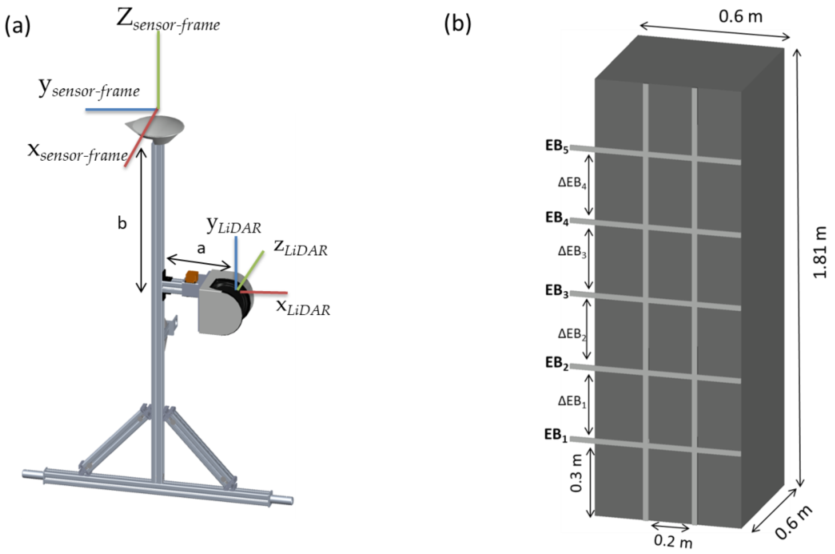
A rigid aluminum sensor-frame carrying the sensors (Figure 1) was mounted on the front three-point-hitch of a tractor. A mobile terrestrial light detection and ranging (LiDAR) (LMS-511, Sick AG, Waldkirch, Germany) laser scanner was mounted at 1.6 m above the ground level. Τwo digital filters were activated to optimize the measured distance values: a fog filter that could not be avoided according to the manufacturer’s setting; and a N-pulse-to-1-pulse filter, which filtered out the first reflected pulse in cases where two pulses were reflected by two objects during a measurement (

Table 1. LMS 511 specification data [25].

Functional Data	General Data
Operating range: up to 10 m	Light detection and ranging (LiDAR) Class: 1 (IEC 60825-1)
Scanning angle: 190°	Enclosure rating: IP 67
Scanning frequency: 25 Hz	Temperature range: −40 °C to 60 °C
Systematic error: ± 25 mm	Light source: 905 nm (near infrared)
Statistical error: ± 6 mm	Total weight: 3.7 kg
Angular resolution: 0.1667°	Laser beam diameter at the front screen: 13.6 mm

).

The three-dimensional tilt of the tractor was monitored by an inertial measurement unit (IMU) MTi-G-710 (XSENS, Enschede, Netherlands), which was placed 0.24 m aside from the LiDAR. The accuracy of the sensor was 1.0° root mean square error (RMSE) for the heading at static and dynamic mode, and 0.25° RMSE and 1.0° RMSE for both pitch and roll in static and dynamic mode, respectively [26]. The measured data was georeferenced by an AgGPS 542 RTK-GNSS (Trimble, Sunnyvale, CA, USA) mounted at 1.74 m height. The horizontal accuracy of the RTK-GNSS was ±25 mm +2 ppm and the vertical ±37 mm +2 ppm.

Software with multi-thread architecture was developed in Visual Studio (version 16.1, Microsoft, Redmond, WA, US) in order to acquire the sensor data. The parallel data acquisition was achieved by creating a dynamic thread for every connected sensor. Consequently, when the raw sensor data were read by each thread, the corresponding measurement and the time stamp from real-time clock (1 ms resolution) were assembled into a text string. The string was stored in a text file for post-processing. The multi-threaded data acquisition of the sensors resulted in non-concurrent measurements. Therefore, the cubic spline interpolation method was used before synchronizing time instances, based on their individual timestamps.

2.3. Sensor-Frame Analysis

A metal box with dimensions 1.81 m × 0.60 m × 0.60 m was constructed to validate the measuring uncertainty of the sensor-frame system (Figure 1b). Five bars with 0.3 m distance from each other were placed horizontally on the metal box. The sensor-frame mounted on a tractor was applied to scan each side of the box separately with 0.13 m s⁻¹. The measurements were carried out next to the apple trees in order to simulate the real-world operating conditions. The mean absolute error (MAE), the bias (MBE) and the RMSE considering the actual and estimated dimensions of the metal box were calculated (Equations (1)–(3))

$$\mathrm{MBE}(\mathrm{mm})=\frac{{{\displaystyle \sum }}_{\mathrm{i}=1}^{\mathrm{n}}\left({\mathrm{D}}_{\mathrm{r},\mathrm{i}}-{\mathrm{D}}_{\mathrm{LiDAR},\mathrm{i}}\right)}{\mathrm{n}}$$

(1)

$$\mathrm{MAE}(\mathrm{mm})=\frac{{{\displaystyle \sum }}_{\mathrm{i}=1}^{\mathrm{n}}\left|{\mathrm{D}}_{\mathrm{r},\mathrm{i}}-{\mathrm{D}}_{\mathrm{LiDAR},\mathrm{i}}\right|}{\mathrm{n}}$$

(2)

$$\mathrm{RMSE}(\%)=\sqrt{\frac{{{\displaystyle \sum }}_{\mathrm{i}=1}^{\mathrm{n}}\left({\mathrm{D}}_{\mathrm{r},\mathrm{i}}{-\mathrm{D}}_{\mathrm{LiDAR},\mathrm{i}}\right)}{\mathrm{n}}}$$

(3)

where D_r,i is the actual reference dimension of the metal box profile, D_LiDAR,i is the dimension of the metal box estimated by the LiDAR for time instance i, and n is the number of the measured points for each profile. Furthermore, the above equations were used to estimate the measuring uncertainty considering the manual and the LiDAR measurements of the stem position, tree height, stem diameter, and canopy volume.

2.4. Data Pre-Processing

The field data were processed using mainly the Computer Vision System Toolbox^TM of Matlab (2017b, MathWorks, Natick, MA, USA), the function of the statistical outlier filter (SOR), and cloud to cloud distance (C2C) of CloudCompare (EDF R&D) for point cloud processing.

The LiDAR data set was filtered for considering only those detections with distance measurements between 0.05 m and 4.00 m. The resulting detections were transformed from polar to Cartesian coordinates (x_LiDAR, y_LiDAR, z_LiDAR). The 3D dynamic tilt orientation (yaw (ψ), pitch (θ), and roll (φ)) of the sensor-frame during the tractor movement was acquired by the IMU sensor in east north up (ENU) local frame. Thus, any point of interest on the sensor-frame could be calculated using coordinate transformation. The position data set, latitude (φ), longitude (λ), and altitude (h) (LLA) obtained by the RTK-GNSS receiver, was expressed in the geodetic frame defined by WGS84.

The RTK-GNSS and the IMU output data had to be converted in the same coordinate system in order to be fused. The fusion was carried out in ENU, since the IMU output data was already in this local coordinate system. However, the RTK-GNSS output data was converted twice, firstly the LLA to earth-centered earth fixed (ECEF) frame and secondly to the ENU frame.

The conversion from the geodetic coordinates to the ECEF coordinates was performed using the following equations [27]

$${\mathrm{x}}_{\mathrm{e}}=\left(\mathsf{\nu }\right(\mathsf{\phi })+\mathrm{h})\cos \left(\mathsf{\phi }\right)\cos \left(\mathsf{\lambda }\right),$$

(4)

$${\mathrm{y}}_{\mathrm{e}}=\left(\mathsf{\nu }\right(\mathsf{\phi })+\mathrm{h})\cos \left(\mathsf{\phi }\right)\sin \left(\mathsf{\lambda }\right),$$

(5)

$${\mathrm{z}}_{\mathrm{e}}{=\left[\mathsf{\nu }\right(\mathsf{\phi }\left)\right(1-\mathrm{e}}^2)+\mathrm{h}]\sin \left(\mathsf{\phi }\right),$$

(6)

where e = 0.0818 is the first numerical eccentricity of the earth ellipsoid, Π_e = [${\mathrm{x}}_{\mathrm{e}}{,\mathrm{y}}_{\mathrm{e}}{,\mathrm{z}}_{\mathrm{e}}$]^T is the position in ECEF coordinates and ν(φ) is the distance from earth’s surface to the z-axis along the ellipsoid normal given by

$$\mathsf{\nu }(\mathsf{\phi })=\frac{\mathsf{\alpha }}{\sqrt{1-{\mathrm{e}}^2{\sin }^2\mathsf{\phi }}}$$

(7)

where α = 6,378,137 m is the semi-major axis length of the earth. The conversion from the ECEF coordinates to the local ENU coordinates was estimated from the equation Π_n = ${\mathrm{T}}_{\mathrm{e}}^{\mathrm{n}}$Π_e, where Π_n = [n, e, d]^T is the position in the local ENU coordinate system, and ${\mathrm{T}}_{\mathrm{e}}^{\mathrm{n}}$ is the transformation matrix from the ECEF to the ENU coordinate system

$${\mathrm{T}}_{\mathrm{e}}^{\mathrm{n}}=\left[\begin{array}{cccc}-\sin \left(\mathsf{\lambda }\right)& \cos \left(\mathsf{\lambda }\right)& 0& 0\\ -\sin \left(\mathsf{\phi }\right)\cos \left(\mathsf{\lambda }\right)& -\sin \left(\mathsf{\phi }\right)\sin \left(\mathsf{\lambda }\right)& \cos \left(\mathsf{\phi }\right)& 0\\ \cos \left(\mathsf{\phi }\right)\cos \left(\mathsf{\lambda }\right)& \sin \left(\mathsf{\lambda }\right)\cos \left(\mathsf{\phi }\right)& \sin \left(\mathsf{\phi }\right)& 0\\ 0& 0& 0& 1\end{array}\right].$$

(8)

The sensor-frame enabled transformations and translation due to the known distances and angles between the sensors. The LiDAR frame was transformed into the RTK-GNSS frame by several translations (Trans (${\mathrm{y}}_{\mathrm{axis}}$, −a) × Trans (${\mathrm{z}}_{\mathrm{axis}}$, +b)) and two rotations (Rot (‘roll’,−$\frac{\mathsf{\pi }}{2}$) × Rot (‘yaw’, −$\frac{\pi }{2}$) in order to georeference each point of the LiDAR

$${[{\mathrm{x}}_{\mathrm{sensor}-\mathrm{frame}},{\mathrm{y}}_{\mathrm{sensor}-\mathrm{frame}},{\mathrm{z}}_{\mathrm{sensor}-\mathrm{frame}}, 1]}^{\mathrm{T}}=[{\mathrm{T}}_{\mathrm{LiDAR}}^{\mathrm{sensor}-\mathrm{frame}}]\times [{\mathrm{x}}_{\mathrm{LiDAR}},{\mathrm{y}}_{\mathrm{LiDAR}},{\mathrm{z}}_{\mathrm{LiDAR}}, 1{]}^{\mathrm{T}}$$

(9)

where ${\mathrm{T}}_{\mathrm{LiDAR}}^{\mathrm{sensor}-\mathrm{frame}}$ is the transformation matrix from the coordinate system of the LiDAR sensor to the coordinate system of the RTK-GNSS

$${\mathrm{T}}_{\mathrm{LiDAR}}^{\mathrm{sensor}-\mathrm{frame}}=\mathrm{Rot}(‘\mathrm{roll}’,-\frac{\mathsf{\pi }}{2})\times \mathrm{Rot}(‘\mathrm{yaw}’,-\frac{\pi }{2})\times \mathrm{Trans}({\mathrm{y}}_{\mathrm{axis}},-\mathrm{a})\times \mathrm{Trans}({\mathrm{z}}_{\mathrm{axis}},+\mathrm{b}).$$

(10)

The general matrix form of all rotations (Rot) and translations (Trans) are shown in Equation (11), and by substituting them in Equation (10), a matrix form representation of the equations can be generated. The three-dimensional tilt orientations were implemented in the point cloud considering the LiDAR timestamp (t).

$$\begin{array}{c}\mathrm{Rot}(‘\mathrm{roll}’,\mathsf{\phi })=\left[\begin{array}{cccc}1& 0& 0& 0\\ 0& {\cos (\mathsf{\phi }}_{\mathrm{t}})& {-\sin (\mathsf{\phi }}_{\mathrm{t}})& 0\\ 0& {\sin (\mathsf{\phi }}_{\mathrm{t}})& {\cos (\mathsf{\phi }}_{\mathrm{t}})& 0\\ 0& 0& 0& 1\end{array}\right],\mathrm{Trans}(‘{\mathrm{x}}_{\mathrm{axis}}’,{\mathrm{x}}_{\mathrm{translation}})=\left[\begin{array}{cccc}1& 0& 0& 0\\ 0& 1& 0& 0\\ 0& 0& 1& 0\\ {\mathrm{x}}_{\mathrm{translation}}& 0& 0& 1\end{array}\right],\\ \mathrm{Rot}(‘\mathrm{pitch}’,\mathsf{\theta })=\left[\begin{array}{cccc}{\cos (\mathsf{\theta }}_{\mathrm{t}})& 0& {\sin (\mathsf{\theta }}_{\mathrm{t}})& 0\\ 0& 1& 0& 0\\ {-\sin (\mathsf{\theta }}_{\mathrm{t}})& 0& {\cos (\mathsf{\theta }}_{\mathrm{t}})& 0\\ 0& 0& 0& 1\end{array}\right],\mathrm{Trans}(‘{\mathrm{y}}_{\mathrm{axis}}’,{\mathrm{y}}_{\mathrm{translation}})=\left[\begin{array}{cccc}1& 0& 0& 0\\ 0& 1& 0& 0\\ 0& 0& 1& 0\\ 0& y_{translation}& 0& 1\end{array}\right],\\ \mathrm{Rot}(‘\mathrm{yaw}’,\mathsf{\psi })=\left[\begin{array}{cccc}\cos ({\psi }_t)& -\sin ({\psi }_t)& 0& 0\\ \sin ({\psi }_t)& \cos ({\psi }_t)& 0& 0\\ 0& 0& 1& 0\\ 0& 0& 0& 1\end{array}\right],\mathrm{Trans}(‘{\mathrm{z}}_{\mathrm{axis}}’,{\mathrm{z}}_{\mathrm{translation}})=\left[\begin{array}{cccc}1& 0& 0& 0\\ 0& 1& 0& 0\\ 0& 0& 1& 0\\ 0& 0& {\mathrm{z}}_{\mathrm{translation}}& 1\end{array}\right]\end{array}$$

(11)

The three-dimensional tilt of the IMU data was implemented to stabilize the orientation of the coordinate system of the sensor-frame (Equation (12))

$${\mathrm{T}}_{\mathrm{LiDAR}}^{\mathrm{ts}-\mathrm{geo}}={\mathrm{T}}_{\mathrm{LiDAR}}^{\mathrm{sensor}-\mathrm{frame}}\times \mathrm{Rot}(‘\mathrm{roll}’,-\mathsf{\phi })\times \mathrm{Rot}(‘\mathrm{pitch}’,-\mathsf{\theta })\times \mathrm{Rot}(‘\mathrm{yaw}’,\mathsf{\psi }).$$

(12)

2.5. Point Cloud Rigid Registration and Stitching

The process started by implementing the SOR filter to each point cloud pair to first compute the average distance of each point to its neighbors and then reject the points that are further than the average distance, while also considering the standard deviation. Furthermore, the random sample consensus (RANSAC) algorithm was used to remove points that belonged to the ground. The distance threshold value between a data point and the plane was defined at 5 mm, while the slope of the field was additionally considered in the plane model through the implementation of the RTK-GNSS height difference of each row. As mentioned above, a plane with 5 mm height was applied in both rows in order to remove the reflectance of the soil. The RANSAC algorithm was applied in each path separately.

The pairwise pathways were pre-aligned due to the aforementioned georeferencing method of point clouds using the RTK-GNSS. An additional rough pre-alignment was carried out in CloudCompare in order to overlap the pair sides in the common coordinate system. The alignment of the pairwise pathways was operated with the iterative closest point algorithm (ICP), which iteratively minimizes the distances of corresponding points. A binary search tree, where each node represents a partition of the k-dimensional space (K-d tree) was used to speed up the ICP process [28]. Moreover, the local surface normal vector and the curvatures were considered as variants in the ICP to select the corresponding point. A weight factor that incorporates the difference of eigenvalues of matched values for the minimization of distances was assigned to x, y, z, and the normal vector. Higher weight was assigned to the x axis, since it was the axis of the driving direction producing the highest deviation between the point cloud pairs. The maximum correspondence distance was set to 0.1 m. Thus, the ICP minimized the distance between a point and the surface of its corresponding point, or the orientation of the normal. Finally, the two sides were merged together into a single point cloud, using a voxel grid filter (1 mm × 1 mm × 1 mm). A similar methodology was followed for the reconstruction of each individual side of the metal box. Initially, a SOR filter was used in order for the point clouds of each individual side to be denoised. Subsequently, the normal vectors and curvatures were estimated and integrated into the ICP algorithm. Thus, the edges of the sides were aligned and later merged. Each side was divided vertically and horizontally into 6 parts using a 0.3 m step in order to acquire the average height and the average width, respectively. The height was measured by the subtraction of maximum and minimum point of each vertical part for each individual side, whereas the width was obtained by the subtraction of maximum and minimum width of each horizontal part.

Furthermore, the height and the width of each individual extended bar (ΕΒ) were measured. The difference of average height between the EB (ΔEB) was estimated, using four vertical planes to obtain the difference between the minimum and maximum point.

2.6. Tree Row Alignment

The methodology for determining the stem position relied on the previous study by Vazquez-Arellano and co-workers [24]. A first-order polynomial curve considering the least absolute residuals (LAR) was used to connect the reference stem positions in each row (Equation (13))

$$y =\alpha \times x +\beta$$

(13)

The slope of the line was utilized by rotating the merged point cloud until it was aligned with the x-axis.

2.7. Tree Stem Estimation

The generated and rotated point clouds were used to acquire 3D point density histograms using a bivariate approach by pairing the x and y values of every point in the point cloud. The bivariate histogram depicts the frequency of points, which fall into each bin of size 3 cm².

A bivariate histogram of the entire row was used to detect the stem position with the highest frequency. A cylinder with the coordinates of the highest peak as a base, with a 0.65 m radius and 4 m height was applied in order to bring a point density histogram within this frame. The point with the highest frequency was considered as the starting point, since it was the one with the highest probability of being a stem. The position of the next stem was estimated in both directions of the x-axis by adding the average intra row distance (0.95 m). At this point, a second cylinder, with the aforementioned dimensions, and the coordinates of the next stem as the center of the base was applied. The point density histogram was used within the cylinder frame to test whether the coordinates of the next stem would remain the same or need to be repositioned. The tree point cloud within the later cylinder was segmented and this process was iteratively applied for all trees of each row.

2.8. Tree Height

When each tree was segmented based on its stem position, the height was estimated by calculating the difference between the maximum and the minimum point in the z-axis (H_LiDAR). However, the plane that was fitted into the soil points with the RANSAC algorithm falsly classified some plant points, which were close to the soil, as soil points [29,30]. Therefore, the rigid transformations used for registering the tree point clouds were implemented to align and merge the soil point clouds. The merged soil point cloud was filtered utilizing the SOR filter, and merged with the tree point cloud. The merged point cloud capturing the tree and soil information was utilized for the height estimation.

2.9. Stem Diameter

As was mentioned above, the S_manual was measured at a height of 0.30 m above the ground for each tree. Thus, the region between 0.05 m and 0.3 m above the soil was selected in each individual segmented tree to calculate the stem diameter (S_LiDAR). The selected points were plotted in x and y-axis. A line connected the points on the boundaries with each other, creating a polygon. The k-means clustering method was applied in order to define the coordinates of the center inside the polygon. Consequently, the maximum Euclidean distance between the center and the boundary points were estimated and compared with the manually measured reference stem diameter.

2.10. Canopy Volume

The H_manual of the tree and distance of the branching point of the tree from the ground were recorded. Canopy width of each tree at height intervals of 0.5 m was measured from both sides. The cross-sectional area of each zone was calculated by multiplying the mean value of the top and bottom width measured with the corresponding height. As was mentioned above, the product of the area and h_manual of the tree was multiplied to determine the V_manual [4].

On the other hand, the convex hull was applied in the segmented tree point clouds. The Delaunnay approach was selected for triangulation, whereas a shrink factor equal to 1 was used to create a compact boundaries that envelops the points. This method fits a boundary around the structure specified and calculates the volume for that region. For measuring volume with this method, an algorithm was developed using the boundary function with same shrink factor accordingly in Matlab [31] to estimate the volume.

3. Results and Discussion

3.1. Measuring Uncertainty of the System Applied in the Field

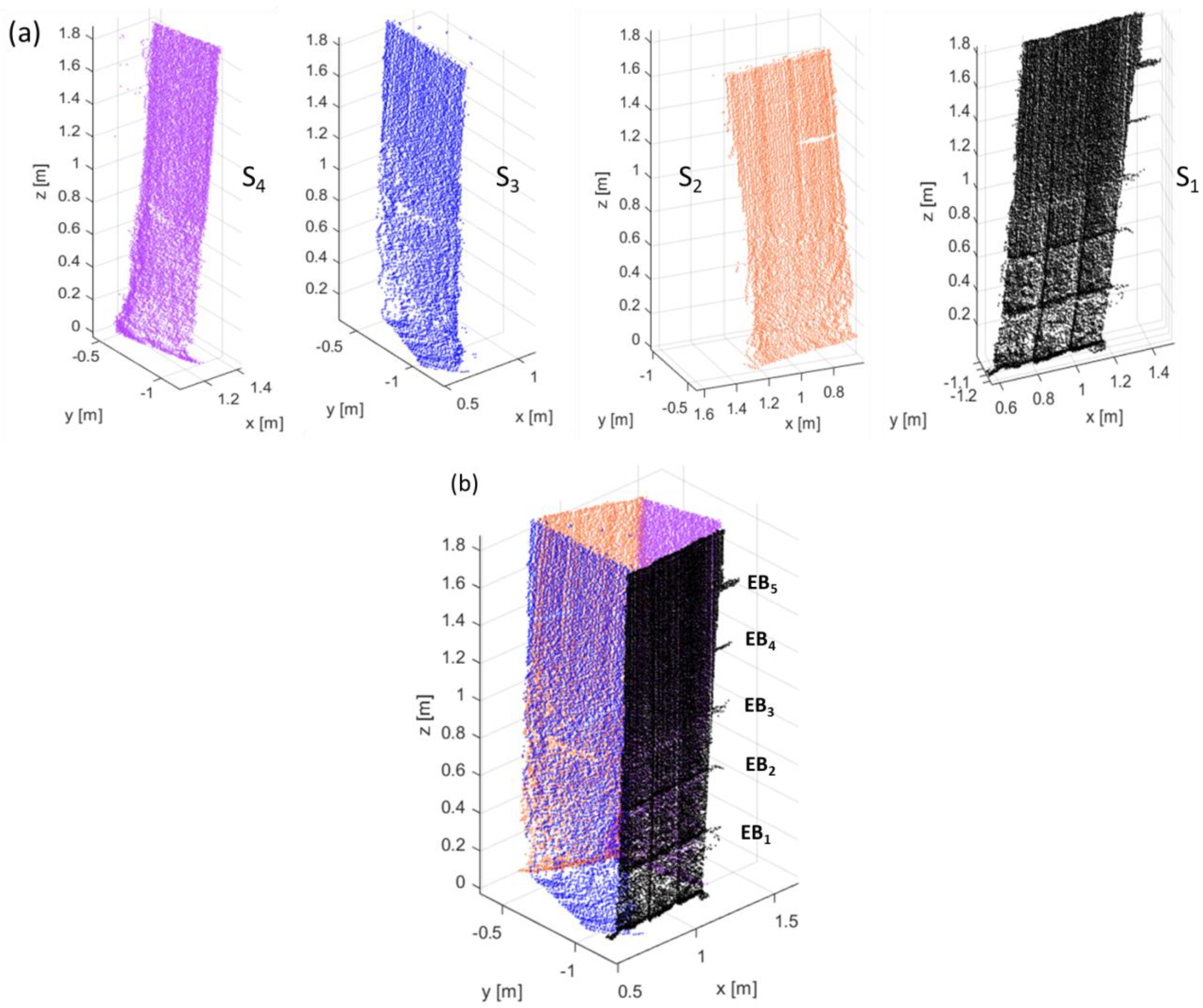
After reconstructing the sides of the metal box, the LiDAR system was able to detect the slope of the soil, and the structural details of the box (Figure 2). The extended metal bars on one side were depicted, whereas their shape was also shown in the main body of S₁. However, gaps of points were visible due to the sun’s reflection from the metal box. The angular resolution of 0.1667° resulted in an average of 20 hits per mm². In total, 565 planes were recorded on S₁, S₃, and S₄ while 643 planes were recorded in S₂. The ICP algorithm was utilized to align and register the sides together and then merged together (Figure 3b). The C2C function was utilized to estimate the average overlapping of the sides, revealing a mean distance error of 12 mm with a standard deviation of 0.5 mm.

The highest MAE and RMSE of height estimation was found for S₁ with 8.18 mm and 1.63%, respectively, while the highest MBE of 2.75 mm was noted at the same side (

Table 2. Height and width results for each side (S) of the metal box (n = 6), maximum (Max), minimum (Min), standard deviation (SD), mean absolute error (MAE), bias (MBE), root mean square error (RMSE).

		Mean (m)	Max (m)	Min (m)	SD (mm)	MAE (mm)	MBE (mm)	RMSE (%)
Height	S1	1.83	1.83	1.81	13.98	8.18	2.75	1.63
	S2	1.80	1.81	1.79	13.34	3.00	1.75	0.60
	S3	1.80	1.82	1.79	1.78	3.31	0.68	0.66
	S4	1.79	1.81	1.79	5.37	1.06	−0.81	0.21
Width	S1	0.60	0.60	0.58	2.10	4.51	2.33	0.90
	S2	0.59	0.60	0.58	7.10	1.50	−1.5	0.30
	S3	0.58	0.59	0.58	7.96	2.06	−4.06	0.81
	S4	0.59	0.61	0.59	8.5	2.18	−2.22	0.43

). For S₄ the lowest MAE and RMSE were depicted with 1.06 mm and 0.21%, respectively. On the other hand, the results of the width showed generally lower MAE, while enhanced MBE were found.

When regarding the extended bars (EB), the S₁ results are becoming more pronounced. The measuring uncertainty increased, when considering the analysis of height and width of EB. EB located closest to the ground, deviating the most from the actual dimensions of the bars (

Table 3. Estimated height and width of the extended bars (EB) (n = 6), maximum (Max), minimum (Min), standard deviation (SD), mean absolute error (MAE), bias (MBE), root mean square error (RMSE).

		Mean (mm)	Max (mm)	Min (mm)	SD (mm)	MAE (mm)	MBE (mm)	RMSE (%)
Height	EB1	21	30	11	7.9	2.1	−2.1	4.2
	EB2	10	30	10	8.5	2.8	−2.8	5.6
	EB3	27	29	20	4.8	0.8	−0.8	1.5
	EB4	28	30	20	4.8	0.6	−1.5	3.2
	EB5	29	30	28	0.9	0.2	−0.2	3.0
Width	EB1	89	100	81	8.5	2.8	2.8	5.5
	EB2	81	85	79	2.6	0.4	−2.8	5.3
	EB3	104	120	85	4.8	0.8	−0.8	1.5
	EB4	102	103	100	1.9	1.5	0.4	0.8
	EB5	102	104	100	1.9	1.6	0.4	0.7

). The EB₄ and EB₅ were closer to the LiDAR height level and less gaps were recognized. Consequently, the measuring uncertainty was reduced. The mean height of EB₅ was 29 mm with the lowest MAE of 0.2 mm and −0.2 mm for the MBE. The highest MBEs of 2.8 mm and −2.8 mm and RMSEs of 5.5% and 5.3% were depicted in EB₁ and EB₂, respectively. Similar results were found by Palleja et al. [15], who mentioned that the LiDAR height misposition due to the roughness of the ground and the oscillations of the tractor engine’s trajectory during the operation can influence the measurement outcome, producing errors of up to 3.5%.

The mean distance between EB₁ and EB₂ (ΔEB₁) was 312.67 mm illustrating, among the other ΔEB, the lowest SD (±1.74 mm) and MAE of 1.27 mm, but also the highest MBE 3.1 mm. Furthermore, the ΔEB₃ deviate the most from the known dimensions of the metal box, with a 293 mm mean and ±6.68 mm SD. It should be mentioned that the mean values of ΔEB₂ and the ΔEB₃ were rather close with 295.2 mm and 296.8 mm, depicting a 4.77 mm and 3.17 mm MBE, respectively.

The scanning process can basically be affected by the scanner mechanism, the atmospheric conditions and environment, the object properties, and the scanning geometry [32]. The highest MBE and MAE have been denoted in the EB measured at a high incident angle. Consequently, the point cloud quality is affected by the scanning geometry, when increased incidence angles and enhanced distances from the scanner occured [33,34]. While the bias may be corrected, the lack of precision remains. It should be also considered that materials of high reflectance can distort the backscattered signal [32]. This was the case for S₃, where 440 missing hits were found. The distortion will be especially pronounced if part of the beam falls outside the target, the likelihood of which additionally depends on the angular resolution [33]. Therefore, the combination of the perturbating factors can possibly increase the MBE and MAE, especially in objects of smaller dimension such as the EB. Whereas this was an expected finding, the quantification points to the measuring uncertainty that can be expected in the analysis of tree stem.

3.2. Separation of Trees by Means of the Stem Position

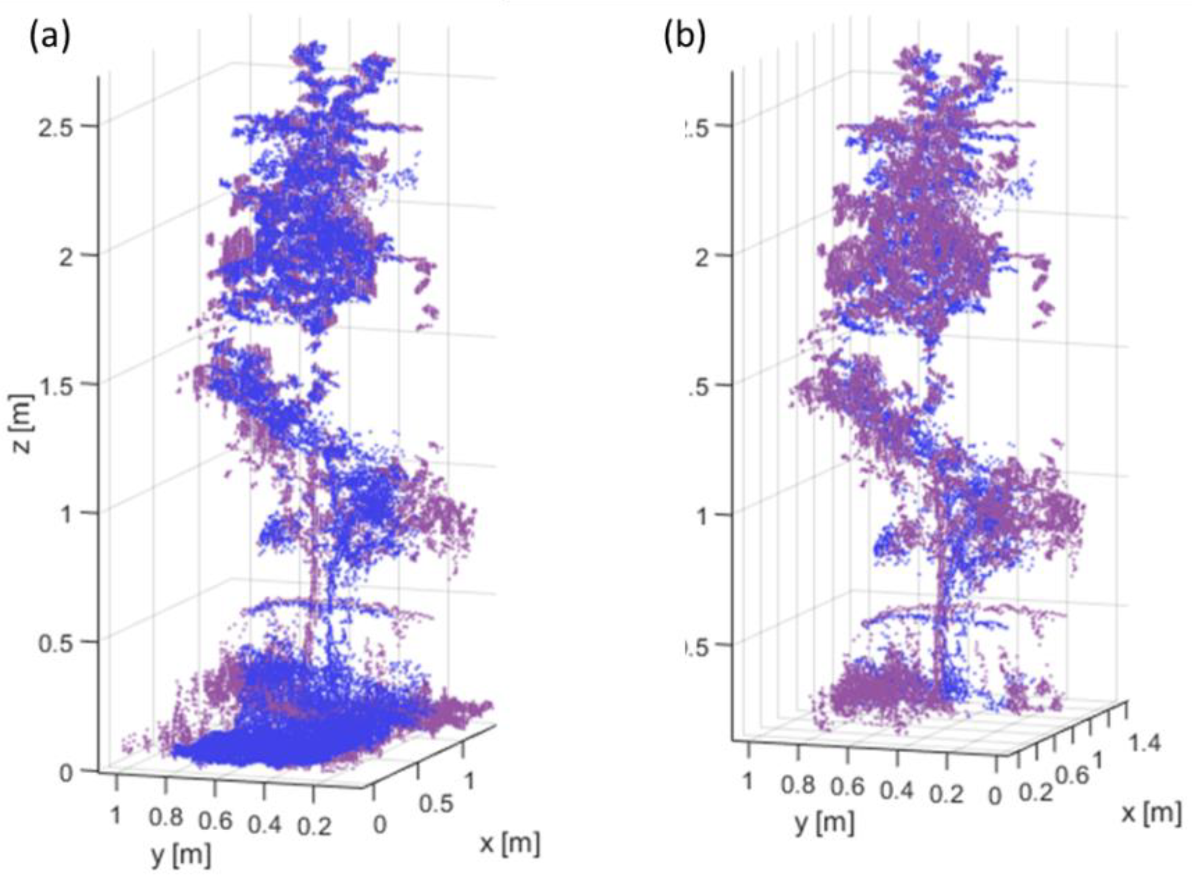
Each side of the row was scanned from both sides by the LiDAR system. The structure of the left side of the trees was described by the a and c pathways, while the right side was described by b and d (Figure 3a,b).

The registration and alignment of the point clouds was carried out pairwise, utilizing the ICP algorithm. The ICP algorithm was utilized in two cases: on the pairwise sides with the soil points (Figure 4a) and on the pairwise sides after the removal of soil points using RANSAC (Figure 4b) in order to evaluate which case provides a better alignment. The C2C function was used to quantify the overlapping differences. Alignment including the soil points resulted in a distance error of 163.5 mm with 31.1 mm SD, and 80.5 mm MBE was observed. The removal of soil points by contrast led to a reduced mean distance error of 81.6 mm with a 21.4 mm SD and lower RMSE of 0.71% as well as an MBE of 5.2 mm. As a result, for the case of the removal of soil points, low measuring uncertainty affecting the overlapping process was found [24,35].

The point clouds of both rows were merged into a single point cloud. The structure of the trees was clearly defined. However, it was observed that weed points above 5 mm remained within the rows (Figure 4b).

The raw data of the 3D reconstructed point cloud consisted of 18,441,933 points. The application of the SOR filter reduced the point cloud by 12.17% removing 2,241,786 points. The segmentation of the soil points using RANSAC algorithm revealed that a further 58.59% of the data (10,820,983 points) belonged to the soil. The remained 5,382,849 points belonged to the trees representing 29.23% of the total amount of points. Arellano and co-workers [30] already pointed out the dominance of soil hits in their 3D reconstructed point clouds, suggesting that the alignment of plant points is separate from the soil points.

The bivariate point density histogram enabled the detection of the peak of laser hits for each individual tree (Figure 5). The assumption that the stem points are concentrated in the center of the plant was based on previous studies [8,24]. Consistently, the area closer to the stem position was assumed to appear with enhanced frequency. However, the assumption needed confirmation considering the formation of the tree canopy and, furthermore, the analysis of number and position of peaks can be affected by the quality of the point cloud. The potential noise or the low quality of overlapping of the point cloud could lead to more peaks since the local bin count becomes more uneven. The use of a stable bin size triggered the filtering of the peaks in the bivariate histogram and, therefore, affected the detection of the highest peak.

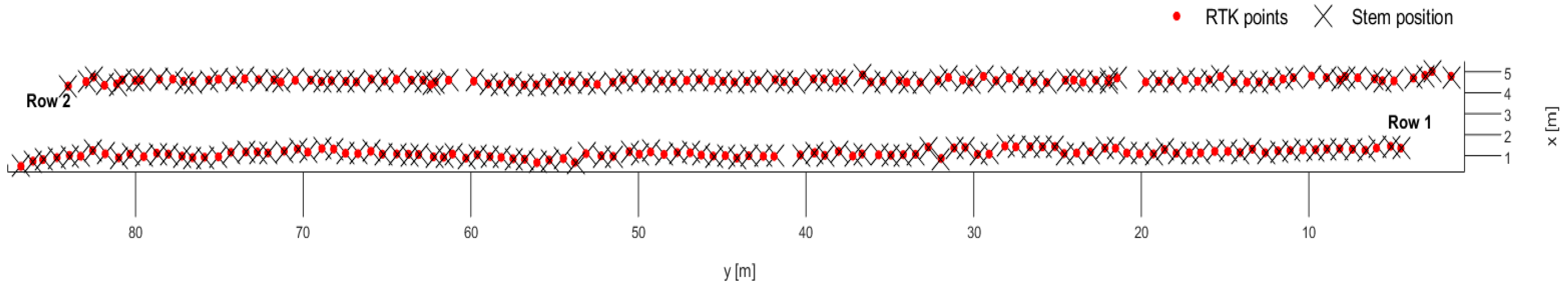
The coordinates of the estimated stem position were compared with the stem position, which was defined with the RTK-GNSS (Figure 6). The estimated stem positions were closely related to the RTK stem positions, revealing 33.7 mm MAE with 36.5 mm MBE. Despite the fact that the alignment occurred with a certain error, the algorithm was able to miss only one stem position out of 224 trees (Figure 6).

3.3. Estimation of Tree Variables

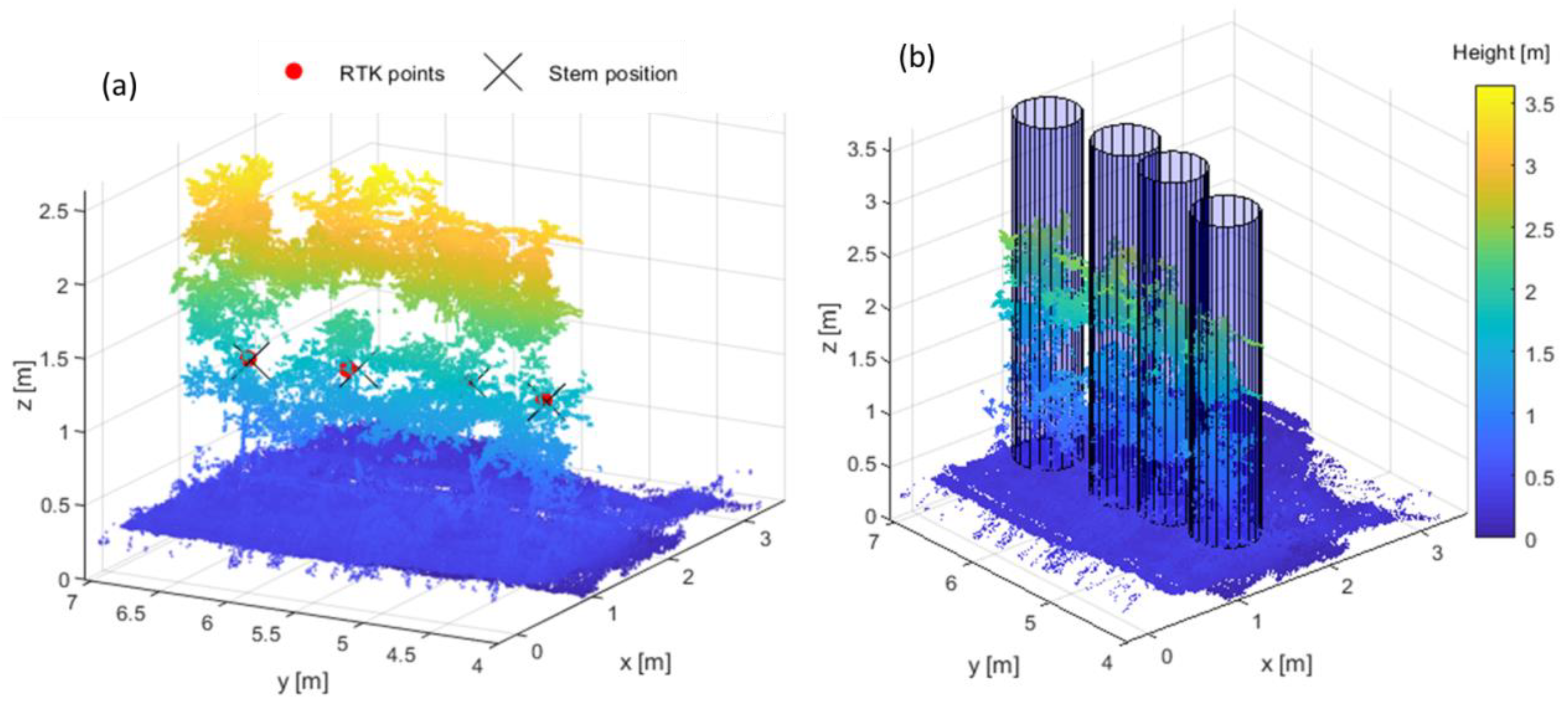
After the determination of stem position, the subtracted soil was merged with the point cloud of trees (Figure 7a) to avoid loosing tree hits. The coordinates of the estimated stem position were utilized as the center for the segmentation cylinders in order to obtain the points that belonged to each individual tree. The points within the boundaries of the cylinder were segmented and considered as the tree points (Figure 7b).

The difference between the maximum and the minimum point in the z-axis was considered to estimate the height. As was mentioned above, the radius of the cylinder was based on the manually measured average width of the trees (n = 224). However, some tree points of long branches were laid out of the cylinder, resulting in an underestimation of the canopy volume. Nevertheless, this error did not reveal an underestimation of the height (

Table 4. Descriptive statistics of manual measurements of height (H_manual) (mm), stem diameter (S_manual) (mm), canopy volume (V_manual) (mm³) and LiDAR-based measurements H_LiDAR, S_LiDAR, V_LiDAR (n = 224) regarding maximum (Max), minimum (Min), mean absolute error (MAE) (mm), bias (MBE) (mm), root mean square error (RMSE), coefficient of determination (R²).

	Min	Max	Mean	MAE	MBE	RMSE (%)	R2
Hmanual (mm)	1900	2800	2310	5.55	0.62	5.71	0.87
HLiDAR (mm)	1870	2820	2350
Smanual (mm)	55	132.5	97.1	2.52	−3.75	2.23	0.88
SLiDAR (mm)	63	136	99.5
Vmanual (m3)	0.23	1.12	0.55	5.23	5.93	4.64	0.77
VLiDAR (m3)	0.38	1.05	0.58

). Arellano et al. [24], with a similar method, determined the stem position in maize and acquired the height profile of the plants pointing to a MAE of 7.3 mm from the actual height. Walnuts trees were segmented and their height was estimated considering the Min and Max values in the z axis, resulting in a significant relationship with the manual measurements (R² = 0.95) [36]. Malambo et al. [37] utilized a similar methodology with cylinder boundaries to segment sorghum trees, reporting a correlation of r = 0.86 with RMSE = 11.4 cm.

In the present study, the plant height profile of each row was measured manually, as the ground-truth in order to validate the results of the point cloud, pointing out a 900 mm variation in height (Table 4). The average values of manual measurements (H_manual) and estimated height, which was derived from LiDAR data (H_LiDAR), varied slightly by 40 mm when comparing the means. Similar values can be expected in commercial apple orchards. The reference and estimated values correlated, revealing an R² = 0.87 with a MAE of 5.55 mm and MBE of 0.62 mm. The RMSE of 5.7% can be explained by the measuring uncertainty of the LiDAR, as well as the uncertainty of defining the highest point of a the stem elongation by means of manual measurements.

The section of stem between 0.10 m and 0.30 m was selected in the segmented tree point clouds to analyse the stem diameter (Figure 8). The grafting region of the cultivar and rootstock appeared always below this section. The S_manual and S_LiDAR depict 2.4 mm difference in their means, whereas an 8 mm difference in minimum values was illustrated. The latter results were described by a considerable difference in the MAE of 2.52 mm and the MBE of −3.75 mm, however, reference and estimated values showed high R² = 0.88 and relatively low 2.23% RMSE recognizing the pertubating effects of enhanced incident angle when measuring on the extended bars of the box (Table 4). The cylinder fitting method based on a stem position for estimating the stem diameter is rather scarce in horticulture. The automatic detection that fits cylinders on stem points, has been investigated broadly in forestry [38,39,40]. However, the majority of these studies employed a 3D terrestrial LiDAR, which is able to provide a 3D representation of stem points without moving the system and as a consequence the limitation of errors during the alignment. Moreover in forests, the tree stem has no coverage from leaves from a few meters above the ground, allowing more hits per stem and segmentation of stem points without imposing coinciding structures.

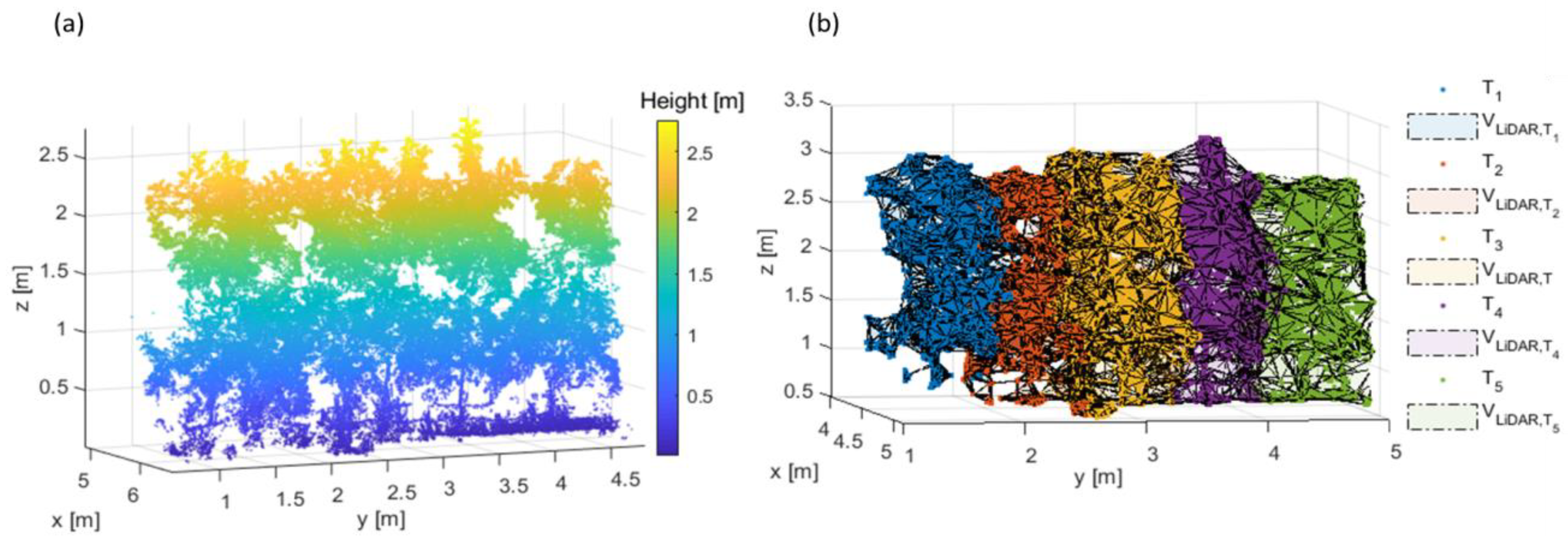
The convex hull algorithm was used to estimate the canopy volume (Figure 9b). The boundary for each individual volume was illustrated in false colour in order to be easily distinct. The convex hull method does not compute volume of the gaps within the canopy, similar to ground-truth methods but instead considers the overall canopy geometry. The manual measurement of the volume showed a strong correlation with the volume data from the segmented tree point clouds (R² = 0.77) (Table 4). The rough simplification of the canopy structure by the manual method based on the cylinder-fit method mainly overestimated the actual data and the ones computed with the convex-hull algorithm. Consequently, the highest bias was found for the volume analysis (Table 4), while a slightly reduced RMSE was observed compared to the height estimation.

This overestimation of volume can be a result of weed points that fall within the cylinder and have not been removed during the soil removal, consequently the convex-hull boundaries were increased which in turn provided an overestimation. In a former study, the convex-hull approach was utilized for the determination of volume in apple trees and vines, revealing a strong correlation of r = 0.81 and r = 0.82, respectively [2]. Furthermore, it was mentioned that the convex-hull approach does not consider the canopy gaps and can lead to an overestiamation. Cheein et al. [13] developed a cylinder based model for real time characterization of volume in apple trees, segmenting the trees based on their canopy center. The model showed 87% accuracy, however the points in the periphery of the cylinder can cause an exaggerated and unrealistic increase in the calculated volume. The methodolology that was proposed in this study for tree segmentation, based on their stem position, revealed a strong relationship between the V_manual and V_LiDAR (R² = 0.77). However, in some trees, the main drawback was that within the cylinder, tree points from neighbor trees interfered, leading to a possible bias of the volume.

4. Conclusions

The LiDAR system was able to estimate a simple structure of objects, with the highest RMSE of 1.63 in a situation with missing hits due to reflectance of the object and an increased incident angle of laser scanner and hit density. Application of a bivariate point density histogram allowed the detection of the tree stem position with an MAE of 43.7 mm and MBE of 36.5 mm. It also provided meaningful information about the H_LiDAR, which correlated strongly with the H_manual (R² = 0.87). Furthermore, the approach for the estimation of S_LiDAR indicated a high relationship with the S_manual (R² = 0.88). The V_manual and the V_LiDAR revealed a lower correlation in comparison with the above parameters (R² = 0.77), probably due to errors in V_manual or the presence of weeds within the trees in the point cloud data. The convex-hull method for estimating the canopy volume was confirmed in apple trees.

Further research needs to be done using clustering algorithms for single plant segmentation (e.g., Euclidian, max-flow/min-cut theorem, region growing segmentation) so that parts of the canopy are not cut off from the tree point cloud, and plants at a later growth stage can be analyzed. Also, non-rigid registration and alignment need to be explored to reduce the effect of the miscellaneous errors that reduce the overlapping between point cloud pairs.

In summary, the LiDAR system was able to detect geometric variables in apple trees that can be used in agricultural applications to measure tree growth for tree-individual orchard management, while considering mechanical pruning, irrigation, and spraying.

References

- Lee, K.H.; Ehsani, R. A laser scanner based measurement system for quantification of citrus tree geometric characteristics. Appl. Eng. Agric. 2009, 25, 777–788. [Google Scholar] [CrossRef]
- Chakraborty, M.; Khot, L.R.; Sankaran, S.; Jacoby, P.W. Evaluation of mobile 3D light detection and ranging based canopy mapping system for tree fruit crops. Comput. Electron. Agric. 2019, 158, 284–293. [Google Scholar] [CrossRef]
- Tsoulias, N.; Paraforos, D.S.; Fountas, S.; Zude-Sasse, M. Calculating the Water Deficit Spatially Using LiDAR Laser Scanner in an Apple Orchard. In Proceedings of the European 12th Conference of Precision Agriculture, Montpellier, France, 8–11 July 2019. [Google Scholar]
- Sanz, R.; Rosell, J.R.; Llorens, J.; Gil, E.; Planas, S. Relationship between tree row LIDAR-volume and leaf area density for fruit orchards and vineyards obtained with a LIDAR 3D Dynamic Measurement System. Agric. For. Meteorol. 2013, 171, 153–162. [Google Scholar] [CrossRef]
- Arno, J.; Escola, A.; Valle’s, J.M.; Llorens, J.; Sanz, R.; Masip, J.; Palacín, J.; Rosell-Polo, J.R. Leaf area index estimation in vineyards using a ground-based LiDAR scanner. Precis. Agric. 2013, 14, 290–306. [Google Scholar] [CrossRef]
- Tagarakis, A.C.; Koundouras, S.; Fountas, S.; Gemtos, T. Evaluation of the use of LIDAR laser scanner to map pruning wood in vineyards and its potential for management zones delineation. Precis. Agric. 2018, 19, 334–347. [Google Scholar] [CrossRef]
- Rosell, J.R.; Sanz, R. A review of methods and applications of the geometric characterization of tree crops in agricultural activities. Comput. Electron. Agric. 2012, 81, 124–141. [Google Scholar] [CrossRef]
- Walklate, P.J.; Cross, J.V.; Richardson, G.M.; Murray, R.A.; Baker, D.E. Comparison of different spray volume deposition models using LIDAR measurements of apple orchards. Biosyst. Eng. 2002, 82, 253–267. [Google Scholar] [CrossRef]
- Rosell Polo, J.R.; Sanz, R.; Llorens, J.; Arnó, J.; Escolà, A.; Ribes-Dasi, M.; Masip, J.; Camp, F.; Gràcia, F.; Solanelles, F.; et al. A tractor-mounted scanning LIDAR for the non-destructive measurement of vegetative volume and surface area of tree-row plantations: A comparison with conventional destructive measurements. Biosyst. Eng. 2009, 102, 128–134. [Google Scholar] [CrossRef]
- Escola, A.; Martínez-Casasnovas, J.A.; Rufat, J.; Arnó, J.; Arbonés, A.; Sebé, F.; Pascual, M.; Sebe, F.; Pascual, M.; Gregorio, E.; et al. Mobile terrestrial laser scanner applications in precision fruticulture/horticulture and tools to extract information from canopy point clouds. Precis. Agric. 2017, 18, 111–132. [Google Scholar] [CrossRef]
- Miranda-Fuentes, A.; Llorens, J.; Gamarra-Diezma, J.; Gil-Ribes, J.; Gil, E. Towards an optimized method of olive tree crown volume measurement. Sensors 2015, 15, 3671–3687. [Google Scholar] [CrossRef] [PubMed]
- Sanz, R.; Llorens, J.; Escolà, A.; Arnó, J.; Planas, S.; Román, C.; Rosell-Polo, J.R. LIDAR and non-LIDAR-based canopy parameters to estimate the leaf area in fruit trees and vineyard. Agric. For. Meteorol. 2018, 260, 229–239. [Google Scholar] [CrossRef]
- Cheein, F.A.A.; Guivant, J.; Sanz, R.; Escolà, A.; Yandún, F.; Torres-Torriti, M.; Rosell-Polo, J.R. Real-time approaches for characterization of fully and partially scanned canopies in groves. Comput. Electron. Agric. 2018, 118, 361–371. [Google Scholar] [CrossRef]
- Colaço, A.F.; Trevisan, R.G.; Molin, J.P.; Rosell-Polo, J.R. Orange tree canopy volume estimation by manual and LiDAR-based methods. Adv. Anim. Biosci. 2017, 8, 477–480. [Google Scholar] [CrossRef]
- Palleja, T.; Tresanchez, M.; Teixido, M.; Sanz, R.; Rosell, J.R.; Palacin, J. Sensitivity of tree volume measurement to trajectory errors from a terrestrial LIDAR scanner. Agric. For. Meteorol. 2010, 150, 1420–1427. [Google Scholar] [CrossRef]
- Jimenez-Berni, J.A.; Deery, D.M.; Rozas-Larraondo, P.; Condon, A.T.G.; Rebetzke, G.J.; James, R.A.; Bovill, W.D.; Sirault, X.R. High throughput determination of plant height, ground cover, and above-ground biomass in wheat with LiDAR. Front. Plant Sci. 2018, 9, 237. [Google Scholar] [CrossRef] [PubMed]
- Escolà, A.; Rosell-Polo, J.R.; Planas, S.; Gil, E.; Pomar, J.; Camp, F.; Solanelles, F. Variable rate sprayer. Part 1—Orchard prototype: Design, implementation and validation. Comput. Electron. Agric. 2013, 95, 122–135. [Google Scholar] [CrossRef]
- Siebers, M.; Edwards, E.; Jimenez-Berni, J.; Thomas, M.; Salim, M.; Walker, R. Fast phenomics in vineyards: Development of GRover, the grapevine rover, and LiDAR for assessing grapevine traits in the field. Sensors 2018, 18, 2924. [Google Scholar] [CrossRef] [PubMed]
- Underwood, J.P.; Jagbrant, G.; Nieto, J.I.; Sukkarieh, S. Lidar-based tree recognition and platform localization in orchards. J. Field Rob. 2015, 32, 1056–1074. [Google Scholar] [CrossRef]
- Reiser, D.; Vázquez-Arellano, M.; Paraforos, D.S.; Garrido-Izard, M.; Griepentrog, H.W. Iterative individual plant clustering in maize with assembled 2D LiDAR data. Comput. Indust. 2018, 99, 42–52. [Google Scholar] [CrossRef]
- Garrido, M.; Perez-Ruiz, M.; Valero, C.; Gliever, C.J.; Hanson, B.D.; Slaughter, D.C. Active optical sensors for tree stem detection and classification in nurseries. Sensors 2014, 14, 10783–10803. [Google Scholar] [CrossRef] [PubMed]
- Zhang, L.; Grift, T.E. A LIDAR-based crop height measurement system for Miscanthus giganteus. Comput. Electron. Agric. 2012, 85, 70–76. [Google Scholar] [CrossRef]
- Sun, S.; Li, C.; Paterson, A. In-field high-throughput phenotyping of cotton plant height using LiDAR. Remote Sens. 2017, 9, 377. [Google Scholar] [CrossRef]
- Vázquez-Arellano, M.; Paraforos, D.S.; Reiser, D.; Garrido-Izard, M.; Griepentrog, H.W. Determination of stem position and height of reconstructed maize plants using a time-of-flight camera. Comput. Electron. Agric. 2018, 154, 276–288. [Google Scholar] [CrossRef]
- SICK AG. Operation Instructions LMS5XX Laser Measurement Sensors. Available online: https://www.sick.com/media/docs/4/14/514/Operating_instructions_Laser_Measurement_Sensors_of_the_LMS5xx_Product_Family_en_IM0037514.pdf (accessed on 21 June 2019).
- Kooi, B. MTi User Manual, MTi 10-Series and MTi 100-Series. 2014. Available online: http://www.farnell.com/datasheets/1935846.pdf (accessed on 21 June 2019).
- Farrell, J.; Barth, M. The Global Positioning System & Inertial Navigation; McGraw-Hill: New York, NY, USA, 1999. [Google Scholar]
- Bentley, J.L. Multidimensional binary search trees used for associative searching. Commun. ACM 1975, 18, 509–517. [Google Scholar] [CrossRef]
- Garrido, M.; Paraforos, D.S.; Reiser, D.; Arellano, M.V.; Griepentrog, H.W.; Valero, C. 3D maize plant reconstruction based on georeferenced overlapping lidar point clouds. Remote Sens. 2015, 7, 17077–17096. [Google Scholar] [CrossRef]
- Vázquez-Arellano, M.; Reiser, D.; Paraforos, D.S.; Garrido-Izard, M.; Burce, M.E.C.; Griepentrog, H.W. 3-D reconstruction of maize plants using a time-of-flight camera. Comput. Electron. Agric. 2018, 145, 235–247. [Google Scholar] [CrossRef]
- Barber, C.B.; Dobkin, D.P.; Huhdanpaa, H.T. The Quickhull Algorithm for Convex Hulls. ACM Trans. Math. Softw. 1996, 22, 469–483. [Google Scholar] [CrossRef]
- Soudarissanane, S.; Lindenbergh, R.; Menenti, M.; Teunissen, P. Scanning geometry: Influencing factor on the quality of terrestrial laser scanning points. ISPRS J. Photogram. Remote Sens. 2011, 66, 389–399. [Google Scholar] [CrossRef]
- Forsman, M.; Börlin, N.; Olofsson, K.; Reese, H.; Holmgren, J. Bias of cylinder diameter estimation from ground-based laser scanners with different beam widths: A simulation study. ISPRS J. Photogram. Remote Sens. 2018, 135, 84–92. [Google Scholar] [CrossRef]
- Kaasalainen, S.; Jaakkola, A.; Kaasalainen, M.; Krooks, A.; Kukko, A. Analysis of incidence angle and distance effects on terrestrial laser scanner intensity: Search for correction methods. Remote Sens. 2011, 3, 2207–2221. [Google Scholar] [CrossRef]
- Lu, H.; Tang, L.; Whitham, S.A.; Mei, Y. A robotic platform for corn seedling morphological traits characterization. Sensors 2017, 17, 2082. [Google Scholar] [CrossRef] [PubMed] [Green Version]
- Estornell, J.; Velázquez-Martí, A.; Fernández-Sarría, A.; López-Cortés, I.; Martí-Gavilá, J.; Salazar, D. Estimation of structural attributes of walnut trees based on terrestrial laser scanning. RAET 2017, 48, 67–76. [Google Scholar] [CrossRef]
- Malambo, L.; Popescu, S.C.; Horne, D.W.; Pugh, N.A.; Rooney, W.L. Automated detection and measurement of individual sorghum panicles using density-based clustering of terrestrial lidar data. ISPRS J Photogramm. Remote Sen. 2019, 149, 1–13. [Google Scholar] [CrossRef]
- Dassot, M.; Colin, A.; Santenoise, P.; Fournier, M.; Constant, T. Terrestrial laser scanning for measuring the solid wood volume, including branches, of adult standing trees in the forest environment. Comput. Electron. Agric. 2012, 89, 86–93. [Google Scholar] [CrossRef]
- Calders, K.; Newnham, G.; Burt, A.; Murphy, S.; Raumonen, P.; Herold, M.; Culvenor, D.; Avitabile, V.; Disney, M.; Armston, J.; et al. Nondestructive estimates of above-ground biomass using terrestrial laser scanning. Methods Ecol. Evol. 2015, 6, 198–208. [Google Scholar] [CrossRef]
- Srinivasan, S.; Popescu, S.; Eriksson, M.; Sheridan, R.; Ku, N.W. Terrestrial laser scanning as an effective tool to retrieve tree level height, crown width, and stem diameter. Remote Sens. 2015, 7, 1877–1896. [Google Scholar] [CrossRef] [Green Version]
Figure 1.
(a) Representation of the sensor-frame system showing the coordinate system of LiDAR and a real time kinematic global navigation satellite system (RTK-GNSS). (b) Metal box of known distances.
Figure 2.
(a) Reconstruction of the four sides from the metal box. S3 and S4 are the sides parallel to the y axis, while S1 and S2 are the sides parallel to the x axis. (b) The resulting merged point cloud after registration and alignment of the four sides of the metal box.
Figure 3.
Representation of the point clouds were reconstructed when the LiDAR system on the tractor drove (a) through the path a, c on the left side and (b) through the path d, b on the right side of apple trees. For illustration purposes, only a part of each row was presented.
Figure 4.
Registration and alignment using the iterative closest point algorithm (ICP) algorithm of a single tree point cloud in two cases (a) tree point cloud with soil points (b) tree point cloud after soil removal with RANSAC. The trees with the best results for each case are presented.
Figure 5.
Result of the registration and alignment of one apple row point cloud after merging and filtering. (a) Intensity image, where the warmer squares indicate the peaks and (b) the bivariate point density histogram of the resulted row point cloud.
Figure 6.
Estimation of the tree (n = 224) stem position compared to the RTK-GNSS defined stem position.
Figure 7.
(a) Merged point cloud with estimated stem position and stem position defined by RTK-GNSS. For illustration purposes, only first part of row 1 is represented. (b) Projected cylinders for single tree segmentation based on the estimated stem position.
Figure 8.
(a) Stem point selection marked in red between 0.1 m and 0.3 m and (b) selected stem points detected by the LiDAR (SLiDAR) plotted in 2D with stem boundaries and stem position.
Figure 9.
(a) Point cloud of four example apple trees and (b) visualization of convex hull method showing the canopy volume (VLiDAR,T) of singularized tree (Tn).