Land-Use Change Modelling in the Upper Blue Nile Basin

Abstract

Land-use and land-cover changes are driving unprecedented changes in ecosystems and environmental processes at different scales. This study was aimed at identifying the potential land-use drivers in the Jedeb catchment of the Abbay basin by combining statistical analysis, field investigation and remote sensing. To do so, a land-use change model was calibrated and evaluated using the SITE (SImulation of Terrestrial Environment) modelling framework. SITE is cellular automata based multi-criteria decision analysis framework for simulating land-use conversion based on socio-economic and environmental factors. Past land-use trajectories (1986–2009) were evaluated using a reference Landsat-derived map (agreement of 84%). Results show that major land-use change drivers in the study area were population, slope, livestock and distances from various infrastructures (roads, markets and water). It was also found that farmers seem to increasingly prefer plantations of trees such as Eucalyptus by replacing croplands perhaps mainly due to declining crop yield, soil fertility and climate variability. Potential future trajectory of land-use change was also predicted under a business-as-usual scenario (2009–2025). Results show that agricultural land will continue to expand from 69.5% in 2009 to 77.5% in 2025 in the catchment albeit at a declining rate when compared with the period from 1986 to 2009. Plantation forest will also increase at a much higher rate, mainly at the expense of natural vegetation, agricultural land and grasslands. This study provides critical information to land-use planners and policy makers for a more effective and proactive management in this highland catchment.

1. Introduction

Current rates, extents and intensities of land-use and land-cover change are driving unprecedented changes in ecosystems and environmental processes at local, regional and global scales. As a result, environmental concerns including climate change, biodiversity loss, land-degradation, soil erosion and pollution of water and air are growing. Interaction of the changes in land use and land cover with various subsystems of the earth system including hydrology, the climate system, biogeochemical cycling, ecological complexity and land degradation make the study of this subject complex [1,2,3,4]. Monitoring and mediating the negative consequences of land-use and land-cover change while sustaining the production of essential resources has therefore become a major priority of researchers and policymakers around the world [5]. However, analyzing the fundamental socio-political, economic, cultural and biophysical forces that may drive land-use and land-cover dynamics and predicting a likely trajectory of future changes constitute one of the main challenges in land-use research [6,7,8]. Land-use modeling is often used for predicting trajectories of future landscapes. A typical approach to land-use change modeling involves investigating how different variables relate to historical land-cover change trends and transitions in the past and use those relationships to build models that project a likely future land-use trajectory [9,10].

The Upper Blue Nile (Abbay) is one of the most diverse and highly important river basins in Ethiopia. The basin faces serious problems including soil erosion, land degradation, loss of soil fertility and deforestation [11,12,13,14]. The major causes are reported to have been a combination of biophysical factors such as seasonal fluctuation in rainfall and climate variability, topographic heterogeneities and anthropogenic factors, e.g., population growth and associated demands that result in soil erosion and land degradation in the basin [15,16,17,18]. Land degradation occurs mainly due to gully and surface erosions by torrential runoff in this rugged highland catchment. No predictive land-use change modeling study addressing socio-economic and biophysical land-use change drivers has yet been reported in the Abbay basin in general and in the Jedeb catchment in particular.

This study is aimed at identifying the potential land-use drivers in the Jedeb catchment of the Abbay basin by combining statistical analysis, field investigation and remote sensing. Potential future trajectory of land-use change was predicted under a business-as-usual scenario in order to provide critical information to land-use planners and policy makers for a more effective and proactive management in the highland catchment. To do so, a land-use change model was developed, calibrated and evaluated using the SITE modelling framework. SITE (SImulation of Terrestrial Environment) is a cellular automata based multi-criteria decision analysis framework for simulating land-use conversion based on socio-economic and environmental factors [19]. (Note that land cover is the observed biophysical cover on the earth's surface whereas land use is characterized by activities and inputs people undertake on land cover type to produce, change or maintain it [20]). In this study, we are simulating changes in land cover using land-use drivers as well as baseline and reference land cover maps.

2. Materials and Methods

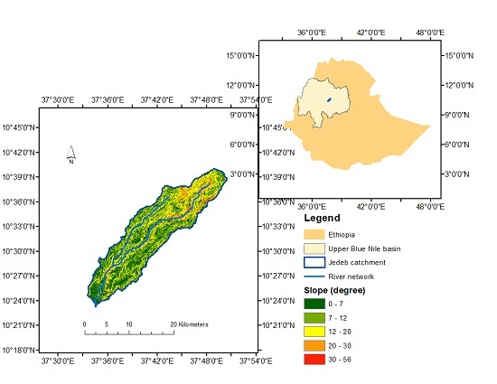
2.1. Study Area

The Jedeb catchment is situated in the south-west part of Mount Choke and it is part of the headwater of the Abbay basin (Figure 1). It covers an area of 297 km² and is situated between 10°22′ to 10°40′ N and 37°33′ to 37°50′ E. The area is known for its diverse topography with elevation extending from 2100 to 4000 m.a.s.l., and slope ranging from nearly flat to very steep (>45°). The mean annual rainfall varies between 1400 and 1600 mm per annum (based on data from three climate stations: Debre Markos, Anjeni and Rob Gebeya). The steep slopes, coupled with erosive rains, have contributed to the excessively high rates of land degradation and soil erosion [21,22]. As one of the severely eroded and degraded parts of the basin, the catchment received the attention of researchers who undertake various socio-environmental and water resources studies in the catchment [23,24]. Land-use and land-cover changes, such as loss of grassland cover due to overgrazing, poor land-use management and change from grassland to agricultural land for instance, may have contributed to a higher level of gully formation, soil erosion and land degradation in general. Between 1957 and 2009, 46% of the watershed has undergone land-use changes without proper soil and water conservation measures in place [25]. The changes in land use and land cover are thought to be among the major causes of high erosion rates in the basin [25,26]. Whether this trend will continue is dependent, among other things, on future land use.

2.2. Conceptual Framework

First, detailed land cover maps for the years 1986 and 2009 derived from Landsat TM Satellite images were used as base and reference (hence forth “observed”) maps for the land-use model, respectively. Then land-use change drivers were identified and the strength of their influence on land-use change estimated by analyzing the spatial correlation between an initial set of potential drivers and land-use types. Rule-sets and initial weights for each deriver variables were developed for each land-use type based on the correlation results. Next, a spatially explicit land-use change model was developed for the SITE modelling framework using the identified land-use drivers and the 1986 land cover map. Based on land-use suitability and historical demands for various land-use types (Section 2.3.4), dynamics of trends of land-use conversion was simulated and analyzed between 1986 and 2009. The simulated output map of 2009 was compared with the reference or observed land cover map of 2009. The model was calibrated based on field data, trend analysis and secondary data sources. Thereafter, the model was used to simulate a business-as-usual scenario of land-use change trajectories of the catchment for the year 2025.

2.3. Inputs and Model Setup

2.3.1. Model Architecture

SITE is a land-use modeling framework based on an extended cellular automata concept, which employs a rule-driven approach on a grid-cell based structure and simulates land-use decisions in annual time steps [19,27]. It is an extended implementation of multi-criteria decision analysis for simulating land-use conversion based on socio-economic and environmental factors. Land-use change is dependent on the defined suitability for each land-cover types, demand for certain land-use classes and neighborhood or proximity factors. Based on demand and suitability, multi-criteria rule-sets are formulated for the cellular automata per land use for the model. It includes modules for calculating suitability and for allocating land-use classes based on suitability. The framework requires a number of Geographic Information System (GIS) based pre-processing of spatial and socio-environmental data. The model inputs include an initial land-cover map and land-use change drivers pre-processed in formats required by the model [19]. Land suitability will be calculated within the suitability module of SITE. This module is subdivided into functions computing biophysical suitability (e.g., elevation, terrain slope, soil fertility) and socio-economic suitability (based on factors such as population, gross margin, accessibility and farmers’ preferences) to produce land suitability maps [19]. All suitability values are normalized to a range between 0 (not suitable) and 1 (perfectly suitable) [27] using Equation (1):

$$S_{kl}=\left(W_B{\displaystyle \sum _{i=1}^m{\beta }_i{S}_{Bikl}+W_E}{\displaystyle \sum _{i=1}^n{\epsilon }_i{S}_{Eikl}}\right)\times {\displaystyle \prod _{j=1}^o{C}_{Bjkl}}{\displaystyle \prod _{j=1}^p{C}_{Ejkl}}$$

(1)

where, W_B + W_E = 1; ${\displaystyle \sum _{i=1}^m{\beta }_i=1}$; ${\displaystyle \sum _{i=1}^n{\epsilon }_i=1}$; and $S_{Bikl}$, $S_{Eikl}$, $C_{Bjkl}$, $C_{Ejkl}$ ∈ [0,1].

The calculation of the overall suitability value S_kl for each land use grid cell k and land-cover types l consists of two terms: the partial suitability S_Bikl for biophysical and S_Eikl for socio-economic factors. C_B and C_E are biophysical and socio-economic constraints, respectively. These factors are weighted using the partial weights ${\beta }_i$/${\epsilon }_i$, where m and n represent the total number of suitability criteria included; whereas o and p represent the total number of biophysical and socio-economic constraints, respectively.

Suitability of land in this implementation is defined by analyzing spatial correlations of where a specific land cover type is found with respect to factors such as slope, elevation, soil, etc., as well as by historically established links between land use and various socio-economic aspects. Each land-cover type, thus, is spatially correlated with a group of attribute sets driving its conversion (such as slope, elevation and proximity to water, road and markets). The allocation module of SITE uses the calculated suitability maps, set of neighborhood functions and defined socio-environmental factors, for allocating land. It follows defined hierarchical priorities and land-use change rules. Suitability factors show what combination of major criteria are suitable for which land cover and hierarchical priorities show which land-cover type takes priority during allocation in case a land parcel is suitable for two or more competing land-cover types.

2.3.2. Land-Use Change Drivers

Potential land-use and land-cover change drivers were gathered through literature review and interviews with key informants including farmers, regional and local land resources administrators and development agents (i.e., government employees assigned in villages to advise farmers on various agro-ecosystems practices, local and regional land administration policies). Land-use practices and perceptions of farmers on issues such as availability of land for various land cover types, perceived changes in the past and their anticipation of future prospects with regards to land use, their practice of crop-rotation and trends and traditions of land-renting were reflected. What the farmers consider as limiting factors of productivity such as access to water for irrigation, roads for transport of products, drought/rainfall limitation and lack of agricultural and grazing land were also deliberated. In addition, regional and national land-use policies, national growth and development plans were consulted. Suitability relevance of distance variables from such as urban centers, water bodies and roads were estimated based on literature and discussions with local experts. The outcome of the discussion with local experts and stakeholders was mainly qualitative, yet has served as a basis for further parameter estimation, in addition to relevant literature, of initial suitability ranges.

Data reduction and correlation analysis between the identified potential drivers and land-uses were conducted using the Principal Component Analysis (PCA) method [28,29]. PCA produces correlations between variables by identifying hidden patterns in data and classifying them according to how much of the information is stored in the data they account for [30]. PCA has been used in literatures to analyze land-cover changes and land-use change drivers [31,32]. Eleven potential land-use drivers (population, distance to market, distance to road, slope, distance to settlement, elevation, livestock, soil type, precipitation, distance to forest edge) and distance to water sources were identified as input to the PCA analysis. By applying the PCA using these driving factors, land-use change drivers that capture most of the variations in change for each land-cover type can be identified. Then, comparative significance (initial suitability weight) for each of the associated land-use change drivers was established using Equation (2). The suitability weights show the importance of each suitability factor in determining the land-cover type.

$$\alpha =\beta /\left({\displaystyle \sum _{i=1}^y{\beta }_i}\right)$$

(2)

where $\alpha$ = comparative significance (initial weight) value; $\beta$ = individual significance value; y = number of significant independent variables for the land-cover type. The quotient of individual significance values and the sum of all the significance values of determinants (land-use drivers) for a land-cover type is a normalized value showing an initial weight between 0 and 1 (Note that in the absence of means of estimation of initial weights for suitability factors on the ground, it is a common practice in SITE to set a default weight of 1 for each suitability subset. This would, however, mean that the model will be forced to “fit” parameters to past observations during calibration irrespective of relevance on the ground). Assignment of an initial weight for calibration reduces the computation burden in addition to serving as a model evaluation tool comparing weights estimated based on ground data against model calibrated values. Initial weights can be altered during model calibration.

2.3.3. Data

Potential land-use change drivers were identified through literature reviews [7,24,33] and field interviews with farmers, local farming experts, regional land bureau officials and through spatial correlations (

Table 1. Data inputs and potential land use change drivers.

Variables	Description	Dataset	Sources *	Scale/Resolution
Population	Gridded population dataset	Census for 1986 & 2007; GPW	CSA, FAO	Sub-district; 1 km
Livestock	Gridded livestock dataset	Gridded livestock (GLW) 2007, 2014	FAO	5 km
Distance to roads	Euclidean distance to major roads	Roads	ERA	30 m
Distance to markets	Euclidean distance to major towns	Markets	FAO-SRDN	30 m
Land cover map	Land cover maps	Landsat TM (1986 & 2009)	Teferi et al [24]	30 m
Settlement maps	Topographic map with settlement locations	Topo1984; Landsat	EMA, GEE	1:50,000; 30 m
Crop map	Map of croplands in the Amhara region	Cultivated land	BoA, MoARD	250 m
Distance to water	Euclidean distance to water sources	Water bodies	MoWE	30 m
Slope and elevation	Elevation (DEM) and slope (derived from DEM)	DEM	USGS	90 m
Soil type	Soil types	Soil group	FAO/FGGD [38]	5 arc min
Precipitation	Average annual precipitation	Precipitation data	MoWE	Annual average
Distance from forest edge	Distance from forest edge	Distance from forest edge	land-use map	30 m

* CSA: Central Statistical Agency of Ethiopia; ERA: Ethiopian Roads Authority; EMA: Ethiopian Mapping Agency; FAO: Food and Agriculture Organization; GLW: Gridded Livestock of the world, an FAO project; GPW= Gridded population of the world; GEE: Google Earth Engine; BoA: Amhara Bureau of Agriculture; MoWE: Ministry of Water & Energy of Ethiopia; EMA: Ethiopian Meteorological Agency; USGS: US Geological Survey; MoARD: Ministry of Agriculture and Rural Development.

). In addition to derived spatial layers such as distances from roads, towns and rivers, a number of biophysical and socio-economic datasets were gathered, pre-processed and used in the land-use model setup (Table 1). Major socio-economic data was collected from the Ethiopian Statistical Agency [34], Atlas of Ethiopian Rural Economy [35] and the Ethiopian Rural Household Survey (1989–2009) [36]. Field observations and interviews with key informants also provided valuable insights in the identification of land-use change drivers in the catchment. The base and reference Landsat Thematic Mapper (TM) based land cover maps for the years 1986 and 2009, respectively, were produced from a previous study carried out in the catchment [24]. The land cover classes were reclassified into 5 groups, i.e., Natural Woody Vegetation (NWV), Plantation Forest (PF), Cultivated Land (CL), Grassland (GL) and Others. To shortly summarize the land-cover classification procedure, a hybrid (supervised and unsupervised) classification approach was adapted with successive GIS/spatial operations. Multispectral pattern recognition using the Iterative Self-Organizing Data Analysis Technique (ISODATA) algorithm [37] was performed on the imageries for the land-cover classification. Field data was collected to associate the spectral classes with the cover types in the classification scheme for the 2009 Landsat imagery. Reference data for the 1986 image was based on aerial photo interpretation of 1982, as well as topographic maps of 1984 at a scale of 1:50,000 collected from the Ethiopian Mapping Agency (EMA). Of a total of 2277 reference data points for the respective years, 759 points were used for accuracy assessment and 1518 points were used for classification. Training sites were developed from the field reference data collected to generate a signature for each land cover type. An overall accuracy of 95.6% and a Kappa coefficient of 0.94 was attained for the 2009 classified map. Similarly, overall classification accuracy of 91.5% (Kappa coefficient of 0.89) was achieved for the 1986 land-cover map (refer Teferi et al. [24] for details on the land-cover classification).

2.3.4. Demand for Land Use

Land-use change is driven by demands for various uses. The demands are associated with livestock and population and thus can be affected by factors at local, regional as well as global scales. Land-use demands include settlements, food production and lifestyle needs; fodder and grazing needs; and/or nature protection/conservation needs, etc. If population increases, one may assume that demands for settlement (especially near urban areas) and cultivation or livestock (in the rural lands) may be higher. Based on case specific information, the amount of added population every year needs to be taken into account and allocated for settlement, cultivation and livestock/grazing requirements. In this case study, human population as well as livestock growth rates were taken from regional datasets, specific demands were estimated based on field investigations and findings from the literature review.

Based on field investigation and the literature, minimum requirements for various land-use types in the catchment were estimated per household,

Table 2. General demand estimations based on Mengistu [41] and Jayne et al. [42].

Variable	Estimated Value
Cultivation requirement	1.17 ha/household
Settlement requirement	0.25 ha/household
Plantation (for fire wood, housing) requirement	0.06 ha/household (about 1/20th of cultivation/household), field survey
Grassland (grazing) requirement	0.25 ha/livestock

The value of 0.25 ha/livestock, estimated by FAO [41], is used for this subsistence production highland catchment which mainly stocks cattle. This value is, therefore, only a cattle-equivalent unit.

. The average number of people in a household is assumed to be the current regional average of 4.3 [39]. Socio-economic demands were estimated based on the projection of the regional growth rates for population and livestock. The historical growth rate for population and livestock for the simulation period were 2.5 % and 1.5% per annum, respectively [34,40]. For instance, demand for settlement or cultivation is expressed based on average individual demands (Table 2). Likewise, demand for grassland is computed based on average livestock demand (Table 2). The demand variables are therefore expressed in terms of population and livestock and their amounts are spatially-explicitly computed in the rule-sets/application codes of SITE. Demand for plantation forest was estimated for households after field investigation.

2.4. Model Evaluation

Initial values for suitability weights and ranges, obtained from the analyses described earlier, were applied to parameterize the model. The initial weight parameters were adjusted by model calibration until a good fit was obtained. The GALib genetic algorithm library [43], which is already embedded in SITE, was used for this purpose. Initial suitability weight parameters for slope, elevation and distance variables (distances from settlement, roads, market and forest edge) were subjected to the calibration algorithm. Land-use change model results are typically evaluated by comparing simulated maps against a reference map. Similarly here, the simulated raster output of the model for 2009 was evaluated against the reference (Landsat derived) map for the same year. Depending on the data structures of the resulting output (raster, vector or hybrid), a number of algorithms have been developed over the years for comparing two maps. However, there does not seem to exist any agreed universal procedure to do that [44]. For a spatially explicit, grid-based categorical data (such as land-use or vegetation classification presented here), cell-by-cell comparison to get the number of matching cells, Equation (3), is often the simplest [45,46].

C_C = N_M/N_T

(3)

where C_C = is coefficient of cell agreement, N_M = number of matched cells, N_T = number of total cells.

Problems with cell-by-cell comparison arise from the fact that if one of the maps is shifted even by a single cell, the agreement of the whole comparison may be compromised. Due to lack of accounting for allocation of the neighborhood cells, a small or even large disagreement can have the same error value. It was progressively noted that a full characterization of a fit between two maps should tackle not only quantity or location of changes of matching cells but also distances between locations of matching cells [44]. To address this and a number of other map comparison bottlenecks [46,47], alternative algorithms have been proposed over the years [48,49,50]. Pontius and Millones [51] suggested that summarizing cross-tabulation matrix of the simulated and the observed land-use map in terms of quantity and spatial allocation disagreements will sufficiently account for differences between two categorical maps in terms of the quantity (changes or persistence) and allocation of matching cells. A variety of statistical summaries of a cross-tabulation matrix tool has been recommended [52]. The cross-tabulation tool provides one comprehensive statistical analysis to answer two important questions simultaneously, that is, how well two maps agree in terms of the quantity of cells in each category and how well they agree in terms of allocation of cells in each category. Equations (4) and (5) represent quantity and allocation disagreements for two categorical maps, respectively [51,53,54].

$$Q_g=({\displaystyle \sum _{i=1}^j{P}_{ig}}-{\displaystyle \sum _{j=1}^j{P}_{gj}})$$

(4)

$$A_g=2Min[({\displaystyle \sum _{i=1}^j{P}_{ig}})-p_{gg},({\displaystyle \sum _{j=1}^j{P}_{gj}})-p_{gg}]$$

(5)

where Q_g = quantity disagreement for category g; A_g = allocation disagreement for category g; j = number of categories; P = proportion of category g.

Quantity disagreement is the difference between two maps due to an imperfect match in overall proportions of all mapped land-cover categories, whereas allocation disagreement is the difference between two maps due to an imperfect match between the spatial allocation of all mapped land-cover categories [51]. Values from the comparison of two maps using this measurement technique range between 1 (100%) (perfect disagreement) and 0 (0%) (perfect agreement). Interpretation of what is a good level of agreement in map comparisons is rather subjective. Landis and Koch [53] lumped possible ranges of map comparison into three groups: agreement value greater than 0.8 (80%) represents strong agreement; agreement value between 0.4 (40%) and 0.8 (80%) represent moderate agreement; and agreement value less than 0.4 (40%) represents poor agreement between two maps. An interpretation by Altman [54] states that comparison agreements are “very good” if two maps agree by more than 0.8 (80%); “good” if they agree 0.6 (60%) to 0.8 (80%); “moderate” if they agree between 0.2 (20%) and 0.6 (60%); and “poor” if they agree by less than 0.2 (20%). In this study, the simulated land-use maps were evaluated against the reference map using the Quantity and Allocation Disagreement measures [51,52].

2.5. Scenario Development

Historical trend analysis of the land-cover changes in the Jedeb shows an increasing demand for plantation forest, due probably to its use as a major source of firewood, lumber, house construction (both for people and for livestock) and various farm tools. This is especially true due to dwindling availability of the natural forests cover in the catchment. Recent regional and local policies prohibit the cutting of trees from natural forests, although this did not seem to have curbed deforestation. During field interviews it was learnt that a series of subsequent years of low yield motivated farmers to prefer planting trees such as Eucalyptus, which grow relatively fast and become a substitute cash earner. These plantation forests are often planted on degraded lands/steep slope area and usually on higher elevation spots such as the hills. Natural woody vegetation exist almost exclusively on the riparian zones of the rivers and streams in the catchment as these are often unreachable and also unusable for other land uses due to deep river gorges and stony soils. Reduction in grassland impacts in particular the farmers with livestock. With growing population and livestock, peripheral grassland areas that were often left unused due to the unfriendly terrain are increasingly being used for cultivation and grazing, thereby exacerbating land degradation and soil erosion. It seems that, at least for the foreseeable future, this trend may not change much, especially with respect to land-use policy and/or demands for the various land-uses. Thus, a business-as-usual scenario for population and livestock growth (and their associated demands for cultivation, settlement and grass/grazing land) was used for simulating the land-use model until 2025. This scenario assumes population and livestock growth rates to continue with the historical growth rates of 2.5 % and 1.5% per year, respectively [34,40]. The choice of 2025 is in line with the country’s long term Growth and Transformation Plans (GTPs) which aims at the nation achieving a middle income status ‘Green Economy’ by 2025 [55].

3. Results and Discussions

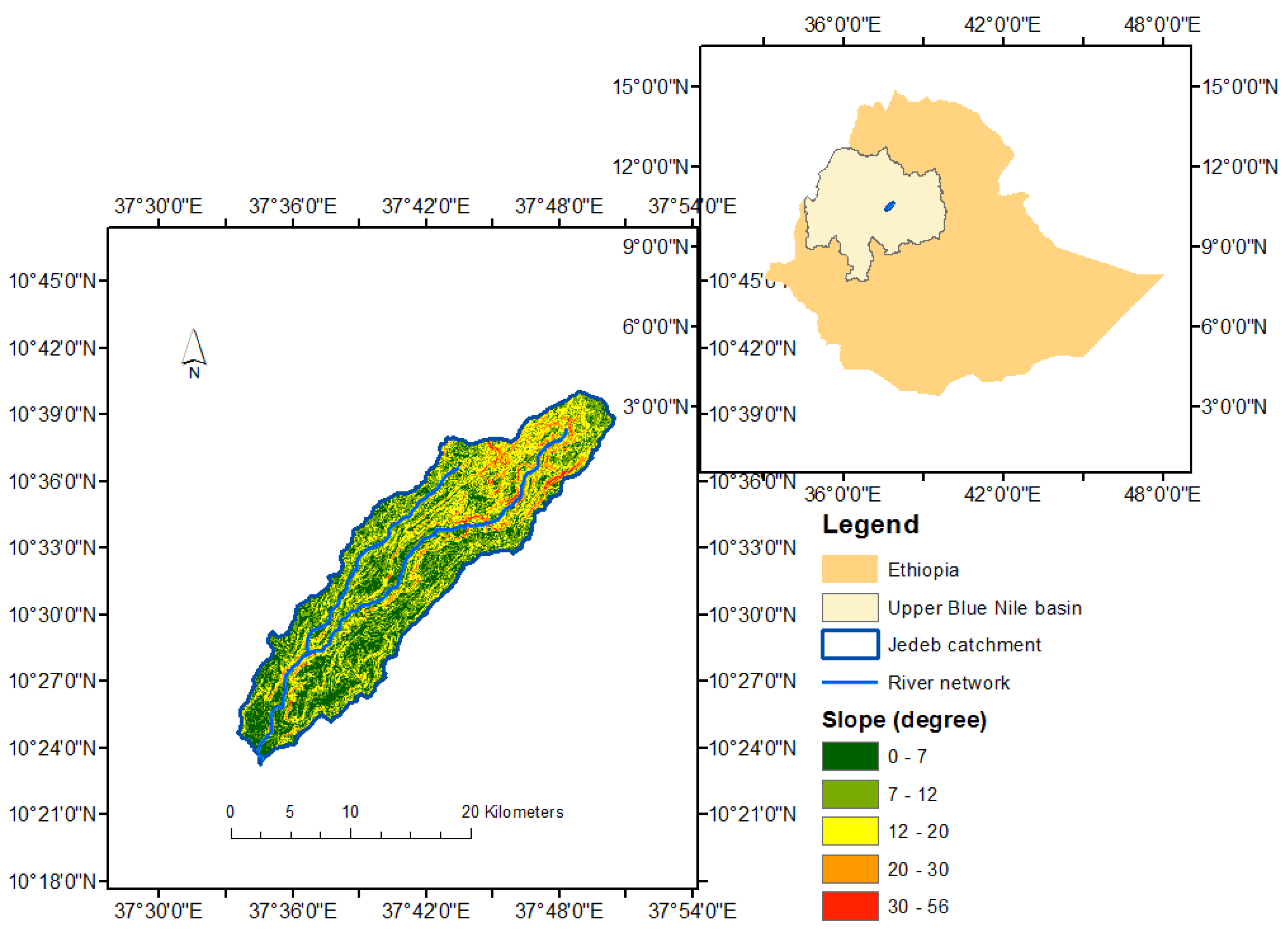
3.1. Land-Use Changes and Drivers

Analysis of changes in land-cover between 1986 and 2009 is shown in

Table 3. Land-use conversion matrix (1986–2009): conversion between land-use classes in km² and percentage of total area (in brackets).

	1986	Natural Woody Vegetation	Plantation Forest	Cultivated Land	Grassland	Others	Total 2009 (km2 (%))
2009
Natural Woody Vegetation		6.59	0.00	2.38	2.05	0.56	11.58
		(2.22)	(0.00)	(0.80)	(0.69)	(0.19)	(3.90)
Plantation Forest		1.40	0.89	3.77	3.86	0.18	10.1
		(0.47)	(0.30)	(1.27)	(1.30)	(0.06)	(3.40)
Cultivated Land		9.50	0.00	150.58	45.07	1.27	206.42
		(3.20)	(0.00)	(50.70)	(15.18)	(0.42)	(69.50)
Grassland		25.84	0.00	4.51	20.87	11.74	62.96
		(8.70)	(0.00)	(1.52)	(7.02)	(4.00)	(21.20)
Others		0.15	0.00	0.33	0.68	4.78	5.94
		(0.05)	(0.00)	(0.11)	(0.23)	(1.60)	(2.00)
Total 1986 (km2 (%))		43.48	0.89	161.57	72.53	18.50	297.00
		(14.64)	(0.30)	(54.40)	(24.42)	(6.20)	(100.00)

. As shown in this table, Cultivated Land and Plantation Forest increased from 54.4% and 0.3% in 1986 to 69.5% and 3.4%, respectively, in 2009 (see also Figure 2). On the other hand, Natural Woody Vegetation and Grassland decreased from 14.6% and 24.4% to 11.6% and 21.2%, respectively, in 2009.

Figure 3 shows map differences/changes comparing 1986 and 2009. From the analysis results shown in Table 3 and Figure 2, major changes were observed between 1986 and 2009, resulting mainly in an increase in Cultivated Land and reduction in Grassland and Natural Woody Vegetation.

The two major land-use change conversions were Natural Woody Vegetation to Grassland (close to 60% of the original woody vegetation has been converted to grassland) and grassland to cultivated land (almost 60% of the original grassland has been converted to cultivated land). On the other hand, land-use classes such as Plantation Forest did not seem to convert to other land-use types during the observed timeframe. Instead it seems that the plantation land-use type continued to expand as farmers increasingly change portions of their plots to Plantation Forest to obtain woodfuel and construction materials, owing to the declining availability of and restrictive local policies on natural forest resources.

Table 4. Summary of significant correlations between land use and driving forces.

	Land Use	Pop.	Slope	Elev.	Dist. to Settlement	Dist. To Roads	Dist. to Market	Livestock	Dist. To Water	Dist. to Forest Edge
Variables
Natural woody vegetation		−0.23	−0.60	0.03	0.08	0.04	−0.01	0.02	0.02	0.84
Plantation forest		0.14	0.69	0.39	−0.52	−0.28	0.02	0.04	0.04	0.01
Cultivated land		0.79	0.65	0.02	−0.26	−0.04	−0.52	0.04	−0.05	0.001
Grassland		−0.40	0.68	0.78	−0.54	−0.03	−0.01	0.23	−0.31	0.04
Others		0.10	0.06	0.001	−0.02	0.01	0.03	0.01	0.10	0.002

Elev. = Elevation; Dist. = Distance.

presents a summary of the correlation results between determinant variables and land-cover types. One can figure out that the land-cover class ”Natural Woody Vegetation” is positively correlated with distances from forest edge and settlement whereas it is negatively correlated with slope and population. Cultivated land correlates strongly with population, slope, distance to market, distance to settlement. Grassland correlates with elevation, slope, distance to settlement, population and distance to water. Plantation Forest shows strong correlation with slope, distance to road, distance to settlement, elevation and population. Similarly, the “others” land use type (which includes urban, bare land and wetlands) has little correlation with population, distance to water and slope.

The PCA method was conducted on the identified eleven potential land-use change drivers to determine the major explanatory variables of the change. Five components with eigenvalues >1 according to Kaiser’s criterion [56] were retained. The rotated component loadings and communality estimates are shown in

Table 5. Factor loadings after varimax rotation and communality estimates (loadings >0.7 are in bold).

LU-Drivers	Rotated Component Loadings					Communality Estimates
	PC1	PC2	PC3	PC4	PC5
Population	0.887	−0.227	0.418	−0.147	0.281	0.946
Distance to market	−0.718	0.005	0.145	−0.020	0.127	0.864
Distance to road	−0.135	0.001	0.889	0.308	0.054	0.885
Slope	0.741	−0.252	0.161	−0.312	0.319	0.939
Elevation	0.010	0.929	0.458	0.208	0.121	0.932
Livestock	0.320	0.721	0.120	0.089	0.073	0.786
Distance to settlement	−0.753	−0.549	−0.644	0.078	−0.057	0.906
Distance to water	−0.247	0.114	0.324	0.096	0.895	0.917
Soil type	0.260	−0.022	0.081	0.069	0.151	0.671
Precipitation	0.253	0.001	0.059	0.066	0.173	0.681
Distance to forest edge	0.078	0.002	0.013	0.921	0.091	0.884
Initial eigenvalues	3.290	1.880	1.810	1.240	1.190	-
Variance (%)	29.910	17.090	16.450	11.270	10.820	-
Cumulative variance (%)	29.910	47.000	63.450	74.730	85.550	-

. The amount of variance in each driver variable that can be explained by the retained five components is represented by the communality estimates. From Table 5, we can see that component 1 (PC1) strongly correlates with population, distance to market, slope and distance to settlement, explaining 29.9% of the variance with high loadings (>0.7). PC2, which correlates with elevation and livestock, explained about 17% of the variance. Distance to road is correlated with PC3, which explains about 16.5% and distance to forest edge is strongly correlated with PC4, which explains about 11.3% of the variance. PC5, which strongly correlates to distance to water, explains about 10.8% of the variance. In combination, the five components explained about 85% of the change (Table 5).

3.2. Land-Use Change Rules

When comparing with the summary of the initial correlations in Table 4, we see that components PC1 to PC5 are correlated with cultivated land, grassland, plantation forest, natural woody vegetation and ”others” land-use types, respectively. The results from the PCA loadings and the correlation table provide the basis for the estimation of parameters of the initial suitability per the land-use types as shown in

Table 6. Suitability rule-sets.

Land Use	Variable	Suitability Ranges	Initial Weight	Assigned Weight (After Calibration)	Direction of Relationship *
Natural and Woody Vegetation	Distance to forest edge	>1000 m	0.35	0.50	Positive
	Distance to Roads	>5000 m	0.25	0.20	Positive
	Slope	<40%	0.20	0.20	Negative
	Distance to settlement	>3000 m	0.20	0.10	Positive
Cultivated land	Slope	<20%	0.40	0.66	-
	Distance to Settlement	<5000 m	0.10	0.20	Negative
	Distance to market	<10,000 m	0.20	0.10	Negative
	Distance to water	<10,000 m	0.30	0.24	Negative
Plantation Forest	Slope	5%–40%	0.20	0.30	-
	Elevation	1200–3400 m	0.20	0.10	-
	Distance to settlement	<5000 m	0.40	0.50	Negative
	Distance to road	<1000 m	0.20	0.10	Positive
Grassland	Slope	>10%	0.30	0.30	Positive
	Elevation	>2600 m.a.s.l.	0.25	0.20	Positive
	Distance to water	<5000 m	0.25	0.30	Negative
	Distance to settlement	<20,000 m	0.20	0.20	Negative

* Negative relationship type shows that as the value of the variable increases and the suitability of the variable for the land-use type will decrease and vice-versa. Positive relationship shows that as the value of the variable increases and the suitability increases as well. This relationship is an interpretation of the correlation analysis result presented in Table 4 and Table 5.

.

Initial weights computed and assigned for each determinant using Equation (2) are shown in the “Initial weight” column in Table 6. Final calibrated weights are given in the “Assigned weight” column. The introduction of initial suitability weight values for the SITE modeling framework puts the model calibration into perspective with respect to field observations. Substantial divergences of calibrated values with initial weights would reveal that a revision of the values might be necessary. Using this procedure, chances for equifinality, a situation where a given state (level of model performance) can be reached by different potential combinations (variations of parameter sets), during model calibration can be avoided or at least minimized. On the other hand, the convergence or the closeness in value of the initial and assigned weights gives a certain level of confidence in model parameterization and in the use of the resulting model setting for future scenario simulations.

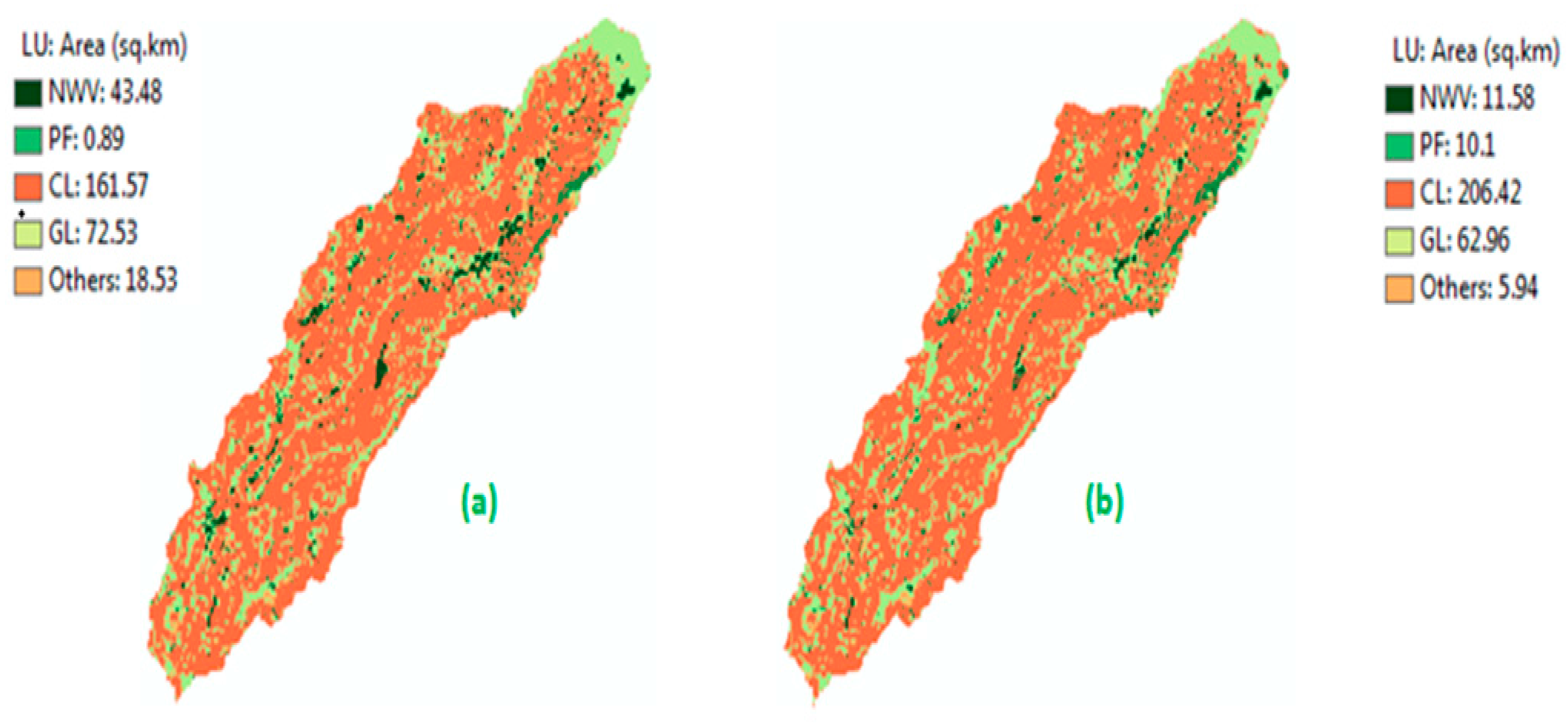
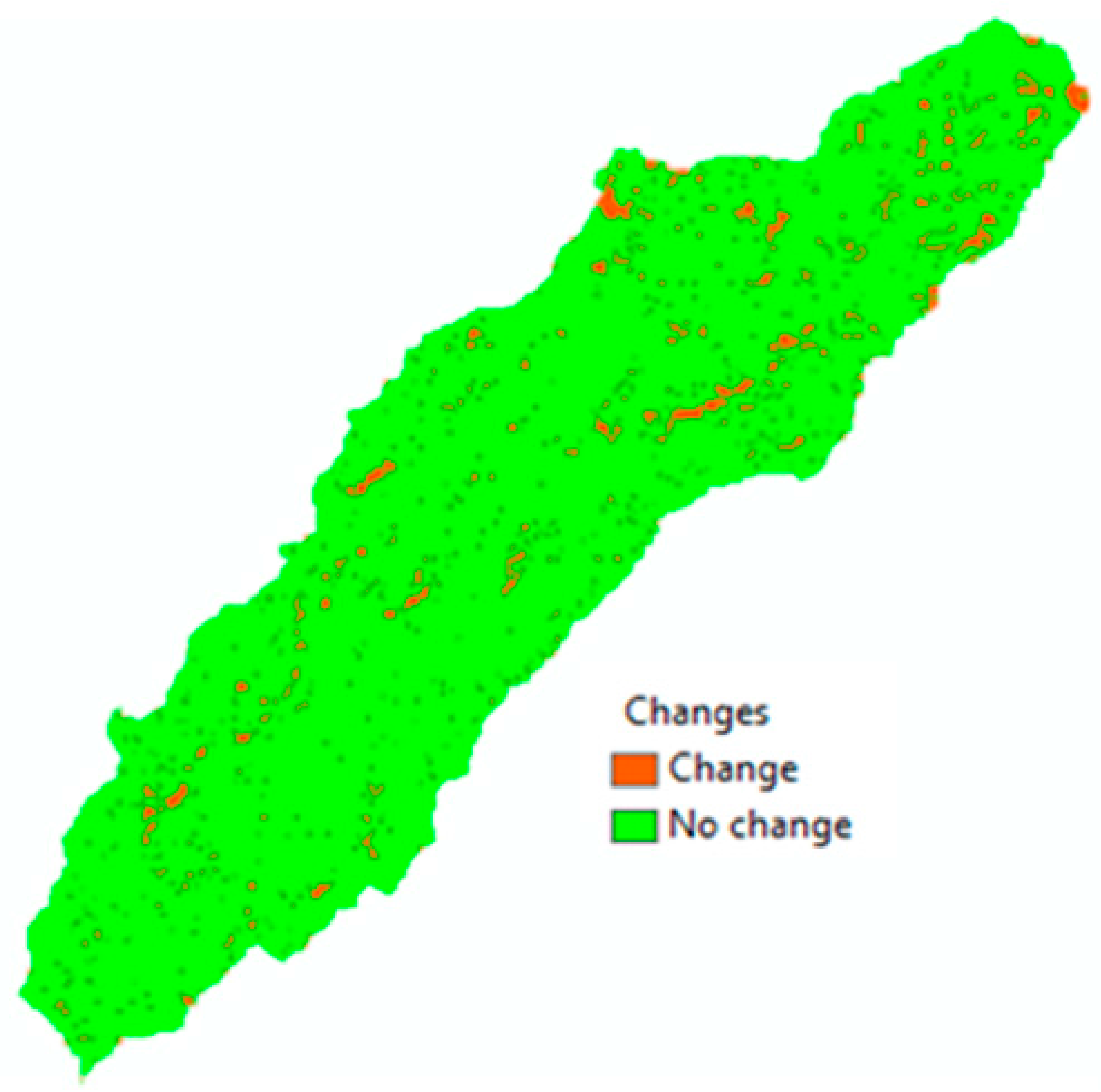
3.3. Model Evaluation

The land-use model was simulated from 1986 to 2009 using the calculated demands, land-use change drivers and the defined rule-sets. The model was calibrated and evaluated using indices of quantity and allocation disagreement measures. Quantity and allocation disagreement between the simulated and the observed cover maps from 2009 show an 8.7% quantity disagreement and a 7.3% allocation disagreement, adding up to a total disagreement of 16% between the two land cover maps (

Table 7. Map comparison indices for the simulated and observed land-cover of 2009.

Name of Algorithm	Component	Measure (%)
Quantity and Allocation Disagreement	Change simulated as “persistence“ (quantity disagreement)	2.5
	Persistence simulated as “change” (quantity disagreement)	6.2
	Change simulated as “change to wrong category” (allocation disagreement)	7.3
	Total Disagreement	16.0

).

From results of the model evaluation shown in Table 7, it was concluded that the simulated land-cover map was able to mimic the major trends both in terms of allocation (spatial) as well as in terms of quantity. Although interpretations on levels of goodness of map comparisons remain still relatively subjective, the evaluation results showed an 84% agreement (more than the 80% threshold discussed previously corresponding to a “very good” agreement). Figure 4 shows results of simulation between 2009 and 2025 and Figure 5 shows the difference maps of the 2009 and 2025 land cover maps.

The simulation results based on BAU scenario show that the expansion of the cultivation land will take about 77% of the total land cover in 2025 (Figure 4;

Table 8. Land-use conversion matrix (2009–2025): total area of conversion between land-cover types in km² and percentages (in brackets).

	2009	Natural Woody Vegetation	Plantation Forest	Cultivated Land	Grassland	Others	Total 2025 (km2 (%))
2025
Natural Woody Vegetation		2.90	0.10	0.23	0.10	0.10	3.40
		(0.98)	(0.03)	(0.08)	(0.03)	(0.03)	(1.15)
Plantation Forest		4.00	8.60	9.39	8.02	0.31	30.30
		(1.35)	(2.90)	(3.16)	(2.7)	(0.10)	(10.20)
Cultivated land		1.80	0.40	196.00	28.34	2.76	229.00
		(0.60)	(0.13)	(66.00)	(9.54)	(0.93)	(77.10)
Grassland		2.10	0.60	0.60	24.90	0.33	28.50
		(0.70)	(0.20)	(0.20)	(8.40)	(0.11)	(9.60)
Others		0.78	0.40	0.20	1.60	2.44	5.40
		(0.26)	(0.13)	(0.07)	(0.50)	(0.82)	(1.82)
Total 2009 (km2 (%))		11.58	10.10	206.42	62.96	5.94	297.00
		(3.90)	(3.40)	(69.50)	(21.20)	(2.00)	(100.00)

). Compared to the period 1986 to 2009 (54 in 1986 and 70 in 2009, see Table 3), the growth rate declines from 200 to 141 ha/year. This may reflect the exhaustion of further suitable land for cultivation based on the defined suitability criteria. It seems likely that the plantation forest area will nearly triple by 2025, most likely at the expense of grassland and cultivated land (Table 8). Coverage of natural woody vegetation and grasslands continue to decline.

The scenario simulations results, as shown in Table 8 and Figure 4, can provide valuable insights on potential implications of land-use management and policy both from a local as well as a regional perspective. First, a continuing decline of natural woody vegetation and grassland implies exacerbation of land degradation and soil erosion in the catchment [57,58]. This can have local consequences such as reduction of environmental and ecological services, thereby impacting crop yields from cultivated lands. Second, the topography of the catchment as the source locations of the Upper Blue Nile River is dominated by rugged and mountainous landscapes. As a result of this, the catchment has been described previously as prone to soil erosion and gully formation [59,60], which has led to a (moderate) decline in soil fertility and loss of fertile plots for local farmers [61,62]. The continuing decline of grasslands and natural vegetation, combined with expanding cultivation, would imply that the local erosion and gully formation phenomenon is bound to deteriorate unless more effective policies and management interventions are developed and implemented. At a more regional scale, consequences of the increase erosion would imply an increased siltation of downstream reservoirs. Simulation of land-use change scenarios and respective analysis, such as the one conducted in this study, may inspire local as well as regional policy makers towards a more sustainable and coordinated regional land and water resources management.

In general, the study showed that in spite of the complexities of involving a wide range of socio-economic and biophysical factors in land-use modelling, the major trends of the past can be captured and reproduced to predict a likely trajectory of land-use change in the Jedeb catchment. As the land-use modeling presented in this study involves various socio-environmental parameters and complexities, a number of uncertainties will likely affect model results. Besides uncertainties pertinent to the land-use model itself, those that propagate with the data gathered and used for the modelling can be expected to affect the certainty of results. We believe that the allocation of initial weight parameters (which are then checked against the assigned weights through calibration afterwards) help to reduce overall uncertainties. With respect to data uncertainties, we have tried to quantify as many of the variables as possible through various spatial correlation techniques in order to reduce subjectivity. Furthermore, where empirical data were lacking, assumptions were made based on the local expert judgments and field observations.

4. Conclusions and Recommendations

Our land-use change model involved complex layers of socio-economic and biophysical factors. With the objective to develop a predictive land-use model, we analyzed socio-economic and biophysical land-use drivers. We developed a land-use change model that was parameterized and calibrated using field data. Based on an initial land cover from 1986, we developed and simulated a land-cover change until 2009. Furthermore, we evaluated and calibrated the simulated map of 2009 with a Landsat derived land cover map for the same year. The study demonstrates methods and techniques for identifying and analyzing land-use change drivers. The simulated map of the year 2009 showed an overall good performance in mimicking land-cover dynamics, trends and magnitudes as confirmed by the observed land cover map. Once evaluated, the simulated model was used to simulate changes until 2025 under a business-as-usual scenario. This scenario assumes present rates of growth in population and livestock as well as associated demands. The fact that no explicit water availability or other water related constraint (except for distances from water bodies) was considered may be one of the limitations of this study that have to be mentioned. Especially in a catchment like that of the Jedeb, where river water is inaccessible (flows in deep gorges), hydrologic components such as surface runoff, ground water storage, and/or evapotranspiration, may be better explanatory variables than the variable distance to water sources. We believe that accounting for hydrologic impacts on the land-use dynamics of this catchment can improve understanding of the catchment land use dynamics further and can be a valuable continuation of this study.

References

1. Fürst, C.; Helming, K.; Lorz, C.; Müller, F.; Verburg, P.H. Integrated land use and regional resource management—A cross-disciplinary dialogue on future perspectives for a sustainable development of regional resources. J. Environ. Manag. 2013, 127, S1–S5. [Google Scholar] [CrossRef] [PubMed]
2. Rindfuss, R.R.; Entwisle, B.; Walsh, S.J.; An, L.; Badenoch, N.; Brown, D.G.; Deadman, P.; Evans, T.P.; Fox, J.; Geoghegan, J. Land use change: Complexity and comparisons. J. Land Use Sci. 2008, 3, 1–10. [Google Scholar] [CrossRef] [PubMed]
3. Halmy, M.W.A.; Gessler, P.E.; Hicke, J.A.; Salem, B.B. Land use/land cover change detection and prediction in the north-western coastal desert of Egypt using Markov-CA. Appl. Geogr. 2015, 63, 101–112. [Google Scholar] [CrossRef]
4. Turner, K.G.; Anderson, S.; Gonzales-Chang, M.; Costanza, R.; Courville, S.; Dalgaard, T.; Dominati, E.; Kubiszewski, I.; Ogilvy, S.; Porfirio, L. A review of methods, data, and models to assess changes in the value of ecosystem services from land degradation and restoration. Ecol. Model. 2016, 319, 190–207. [Google Scholar] [CrossRef]
5. Ellis, E.; Pontius, R. Land-use and land-cover change. In Encyclopedia of Earth; Springer: Washington, DC, USA, 2007. [Google Scholar]
6. Geist, H.J.; Lambin, E.F. Proximate Causes and Underlying Driving Forces of Tropical Deforestation: Tropical forests are disappearing as the result of many pressures, both local and regional, acting in various combinations in different geographical locations. BioScience 2002, 52, 143–150. [Google Scholar] [CrossRef]
7. Veldkamp, A.; Lambin, E.F. Predicting land-use change. Agric. Ecosyst. Environ. 2001, 85, 1–6. [Google Scholar] [CrossRef]
8. Rendana, M.; Rahim, S.A.; Idris, W.M. R.; Lihan, T.; Rahman, Z.A. CA-Markov for Predicting Land Use Changes in Tropical Catchment Area: A Case Study in Cameron Highland, Malaysia. J. Appl. Sci. 2015, 15, 689. [Google Scholar] [CrossRef]
9. Chen, H.; Pontius, R.G., Jr. Diagnostic tools to evaluate a spatial land change projection along a gradient of an explanatory variable. Landsc. Ecol. 2010, 25, 1319–1331. [Google Scholar] [CrossRef]
10. Pontius, R.G., Jr.; Boersma, W.; Castella, J.-C.; Clarke, K.; de Nijs, T.; Dietzel, C.; Duan, Z.; Fotsing, E.; Goldstein, N.; Kok, K. Comparing the input, output, and validation maps for several models of land change. Ann. Reg. Sci. 2008, 42, 11–37. [Google Scholar] [CrossRef]
11. Asres, R.S.; Tilahun, S.A.; Ayele, G.T.; Melesse, A.M. Analyses of Land Use/Land Cover Change Dynamics in the Upland Watersheds of Upper Blue Nile Basin. In Landscape Dynamics, Soils and Hydrological Processes in Varied Climates; Springer: Berlin, Germany, 2016; pp. 73–91. [Google Scholar]
12. Abegaz, A.; Winowiecki, L.A.; Vågen, T.-G.; Langan, S.; Smith, J.U. Spatial and temporal dynamics of soil organic carbon in landscapes of the upper Blue Nile Basin of the Ethiopian Highlands. Agric. Ecosyst. Environ. 2016, 218, 190–208. [Google Scholar] [CrossRef]
13. Jørgensen, L. Advances in Stated Preference Studies for Valuing and Managing the Environment—A Developing Country Context. Ph.D. Thesis, University of Copenhagen, København, Denmark, 23 November 2015. [Google Scholar]
14. Tesfaye, A.; Negatu, W.; Brouwer, R.; Zaag, P. Understanding soil conservation decision of farmers in the Gedeb watershed, Ethiopia. Land Degrad. Dev. 2014, 25, 71–79. [Google Scholar] [CrossRef]
15. Bewket, W. Land cover dynamics since the 1950s in Chemoga watershed, Blue Nile basin, Ethiopia. Mt. Res. Dev. 2002, 22, 263–269. [Google Scholar] [CrossRef]
16. Hurni, H.; Tato, K.; Zeleke, G. The implications of changes in population, land use, and land management for surface runoff in the upper Nile basin area of Ethiopia. Mt. Res. Dev. 2005, 25, 147–154. [Google Scholar] [CrossRef]
17. Steenhuis, T.S.; Collick, A.S.; Easton, Z.M.; Leggesse, E.S.; Bayabil, H.K.; White, E.D.; Awulachew, S.B.; Adgo, E.; Ahmed, A.A. Predicting discharge and sediment for the Abay (Blue Nile) with a simple model. Hydrol. Process. 2009, 23, 3728–3737. [Google Scholar] [CrossRef]
18. Setegn, S.G.; Srinivasan, R.; Dargahi, B.; Melesse, A.M. Spatial delineation of soil erosion vulnerability in the Lake Tana Basin, Ethiopia. Hydrol. Process. 2009, 23, 3738. [Google Scholar] [CrossRef]
19. Schweitzer, C.; Priess, J.A.; Das, S. A generic framework for land-use modelling. Environ. Model. Softw. 2011, 26, 1052–1055. [Google Scholar] [CrossRef]
20. Di Gregorio, A. Land Cover Classification System: Classification Concepts and User Manual: LCCS; Food and Agriculture Organization of the United Nationsb (FAO): Rome, Italy, 2005. [Google Scholar]
21. Easton, Z.; Fuka, D.; White, E.; Collick, A.; Biruk Ashagre, B.; McCartney, M.; Awulachew, S.; Ahmed, A.; Steenhuis, T. A multi basin SWAT model analysis of runoff and sedimentation in the Blue Nile, Ethiopia. Hydrol. Earth Syst. Sci. 2010, 14, 1827–1841. [Google Scholar] [CrossRef]
22. Betrie, G.; Mohamed, Y.; Griensven, A.V.; Srinivasan, R. Sediment management modelling in the Blue Nile Basin using SWAT model. Hydrol. Earth Syst. Sci. 2011, 15, 807–818. [Google Scholar] [CrossRef]
23. Tesfaye, A.; Brouwer, R. Testing participation constraints in contract design for sustainable soil conservation in Ethiopia. Ecol. Econ. 2012, 73, 168–178. [Google Scholar] [CrossRef]
24. Teferi, E.; Bewket, W.; Uhlenbrook, S.; Wenninger, J. Understanding recent land use and land cover dynamics in the source region of the Upper Blue Nile, Ethiopia: Spatially explicit statistical modeling of systematic transitions. Agric. Ecosyst. Environ. 2013, 165, 98–117. [Google Scholar] [CrossRef]
25. Bewket, W.; Teferi, E. Assessment of soil erosion hazard and prioritization for treatment at the watershed level: Case study in the Chemoga watershed, Blue Nile Basin, Ethiopia. Land Degrad. Dev. 2009, 20, 609–622. [Google Scholar] [CrossRef]
26. Pankhurst, A. Land Degradation. In Water Resources Management in Ethiopia: Implications for the Nile Basin; Cambria Press: Amherst, NY, USA, 2010; Volume 213. [Google Scholar]
27. Mimler, M.; Priess, J.A. Design and Complementation of a Generic Modeling Framework—A Platform for Integrated Land Use Modeling; Kassel University Press GmbH: Kassel, Germany, 2008. [Google Scholar]
28. Abdi, H.; Williams, L.J. Principal component analysis. Wiley Interdiscip. Rev. Comput. Stat. 2010, 2, 433–459. [Google Scholar] [CrossRef]
29. Abdi, H. Factor rotations in factor analyses. In Encyclopedia for Research Methods for the Social Sciences; Sage: Thousand Oaks, CA, USA, 2003; pp. 792–795. [Google Scholar]
30. Jolliffe, I. Principal Component Analysis; Wiley Online Library: Hoboken, NJ, USA, 2005. [Google Scholar]
31. Du, X.; Jin, X.; Yang, X.; Yang, X.; Zhou, Y. Spatial pattern of land use change and its driving force in Jiangsu Province. Int. J. Environ. Res. Public Health 2014, 11, 3215–3232. [Google Scholar] [CrossRef] [PubMed]
32. Skånes, H.; Bunce, R. Directions of landscape change (1741–1993) in Virestad, Sweden—Characterised by multivariate analysis. Landsc. Urban Plan. 1997, 38, 61–75. [Google Scholar] [CrossRef]
33. Serneels, S.; Lambin, E.F. Proximate causes of land-use change in Narok District, Kenya: A spatial statistical model. Agric. Ecosyst. Environ. 2001, 85, 65–81. [Google Scholar] [CrossRef]
34. Central Statistical Agency (CSA). Population and Housing Census of Ethiopia; CSA: Addis Ababa, Ethiopia, 2007.
35. Chamberlin, J.; Tadesse, M.; Benson, T.; Zakaria, S. An Atlas of the Ethiopian Rural Economy: Expanding the range of available information for development planning. Inform. Dev. 2007, 23, 181–192. [Google Scholar] [CrossRef]
36. Dercon, S.; Hoddinott, J. The Ethiopian Rural Household Surveys: Introduction; International Food Policy Research Institute: Washington, DC, USA, 2004. [Google Scholar]
37. Ball, G.H.; Hall, D.J. ISODATA, a Novel Method of Data Analysis and Pattern Classification; DTIC Document: Menlo Park, CA, USA, 1965. [Google Scholar]
38. FAO. GEONETWORK: Major Soil Groups of the World (FGGD); FAO: Rome, Italy, 2013. [Google Scholar]
39. CSA. Summary and Statistical Report of the 2007 Population and Housing Census; Federal Democratic Republic of Ethiopia: Addis Ababa, Ethiopia, 2008.
40. FAO. Livestock Sector Brief: Ethiopia; FAO, Livestock Information, Sector Analysis and Policy Branch AGAL: Rome, Italy, 2004. [Google Scholar]
41. Mengistu, A. Country Pasture/Forage Resource Profiles of Ethiopia; FAO: Rome, Italy, 2006. [Google Scholar]
42. Jayne, T.S.; Yamano, T.; Weber, M.T.; Tschirley, D.; Benfica, R.; Chapoto, A.; Zulu, B. Smallholder income and land distribution in Africa: Implications for poverty reduction strategies. Food Policy 2003, 28, 253–275. [Google Scholar] [CrossRef]
43. Wall, M. GAlib: A C++ library of genetic algorithm components. Mech. Eng. Dep. Mass. Inst. Technol. 1996, 87, 54. [Google Scholar]
44. Kuhnert, M.; Voinov, A.; Seppelt, R. Comparing raster map comparison algorithms for spatial modeling and analysis. Photogramm. Eng. Remote Sens. 2005, 71, 975. [Google Scholar] [CrossRef]
45. Visser, H.; de Nijs, T. The map comparison kit. Environ. Model. Softw. 2006, 21, 346–358. [Google Scholar] [CrossRef]
46. Pontius, R.G.; Shusas, E.; McEachern, M. Detecting important categorical land changes while accounting for persistence. Agric. Ecosyst. Environ. 2004, 101, 251–268. [Google Scholar] [CrossRef]
47. Hagen-Zanker, A.; Lajoie, G. Neutral models of landscape change as benchmarks in the assessment of model performance. Landsc. Urban Plan. 2008, 86, 284–296. [Google Scholar] [CrossRef] [Green Version]
48. Van Vliet, J.; Hagen-Zanker, A.; Hurkens, J.; van Delden, H. A fuzzy set approach to assess the predictive accuracy of land use simulations. Ecol. Model. 2013, 261, 32–42. [Google Scholar] [CrossRef]
49. Van Vliet, J.; Bregt, A.K.; Hagen-Zanker, A. Revisiting Kappa to account for change in the accuracy assessment of land-use change models. Ecol. Model. 2011, 222, 1367–1375. [Google Scholar] [CrossRef]
50. Pontius, R.G., Jr.; Peethambaram, S.; Castella, J.-C. Comparison of three maps at multiple resolutions: A case study of land change simulation in Cho Don District, Vietnam. Ann. Assoc. Am. Geogr. 2011, 101, 45–62. [Google Scholar] [CrossRef]
51. Pontius, R.G., Jr.; Millones, M. Death to Kappa: Birth of quantity disagreement and allocation disagreement for accuracy assessment. Int. J. Remote Sens. 2011, 32, 4407–4429. [Google Scholar] [CrossRef]
52. Olmedo, M.T.C.; Pontius, R.G.; Paegelow, M.; Mas, J.-F. Comparison of simulation models in terms of quantity and allocation of land change. Environ. Model. Softw. 2015, 69, 214–221. [Google Scholar] [CrossRef]
53. Landis, J.R.; Koch, G.G. The measurement of observer agreement for categorical data. Biometrics 1977, 33, 159–174. [Google Scholar] [CrossRef] [PubMed]
54. Altman, D. Comparing groups—Categorical data. Pract. Stat. Med. Res. 1991, 1, 261–265. [Google Scholar]
55. FDRE REDD: Proposal Submitted to Forest Carbon Partnership Facility; Forest Carbon Partnership Facility (FCPF): Washington, DC, USA, 2011.
56. Kaiser, H.F. The application of electronic computers to factor analysis. Educ. Psychol. Meas. 1960, 20, 141–151. [Google Scholar] [CrossRef]
57. Simane, B.; Zaitchik, B.F.; Ozdogan, M. Agroecosystem analysis of the Choke Mountain watersheds, Ethiopia. Sustainability 2013, 5, 592–616. [Google Scholar] [CrossRef]
58. Bewket, W.; Abebe, S. Land-use and land-cover change and its environmental implications in a tropical highland watershed, Ethiopia. Int. J. Environ. Stud. 2013, 70, 126–139. [Google Scholar] [CrossRef]
59. Tekleab, S.; Wenninger, J.; Uhlenbrook, S. Characterisation of stable isotopes to identify residence times and runoff components in two meso-scale catchments in the Abay/Upper Blue Nile basin, Ethiopia. Hydrol. Earth Syst. Sci. 2014, 18, 2415–2431. [Google Scholar] [CrossRef] [Green Version]
60. Tekleab, S.; Mohamed, Y.; Uhlenbrook, S.; Wenninger, J. Hydrologic responses to land cover change: The case of Jedeb mesoscale catchment, Abay/Upper Blue Nile basin, Ethiopia. Hydrol. Process. 2014, 28, 5149–5161. [Google Scholar] [CrossRef]
61. Haregeweyn, N.; Tsunekawa, A.; Tsubo, M.; Meshesha, D.; Adgo, E.; Poesen, J.; Schütt, B. Analyzing the hydrologic effects of region-wide land and water development interventions: A case study of the Upper Blue Nile basin. Reg. Environ. Chang. 2016, 16, 951–966. [Google Scholar] [CrossRef]
62. Zeleke, G.; Hurni, H. Implications of land use and land cover dynamics for mountain resource degradation in the Northwestern Ethiopian highlands. Mount. Res. Dev. 2001, 21, 184–191. [Google Scholar] [CrossRef]
Figure 1. Location and topographic map of the Jedeb catchment in the Abbay (Upper Blue Nile) basin, Ethiopia.
Environments 03 00021 g001
Figure 2. Observed land-use maps of (a) 1986 and (b) 2009.
Environments 03 00021 g002
Figure 3. Changes between observed maps of 2009 and 1986.
Environments 03 00021 g003
Figure 4. Simulated land-use maps of (a) 2009 and (b) 2025.
Environments 03 00021 g004
Figure 5. Difference map of (a) observed and simulated maps of 2009 and (b) simulated maps of 2009 and 2025.
Environments 03 00021 g005