
Drivers of Plot-Scale Variability of CH4 Consumption in a Well-Aerated Pine Forest Soil


1
Chair of Soil Ecology, Institute of Forest Science, University of Freiburg, Freiburg 79098, Germany
2
School of Ecosystem and Forest Science, Faculty of Science, Burnley Campus, The University of Melbourne, Melbourne, VIC 3121, Australia
*
Author to whom correspondence should be addressed.
Forests 2017, 8(6), 193; https://doi.org/10.3390/f8060193
Submission received: 7 April 2017
/
Revised: 30 May 2017
/
Accepted: 31 May 2017
/
Published: 3 June 2017
(This article belongs to the Special Issue Forest Soil Microbe and Biogeochemical Cycling: Biogeochemical Processes in Forest Soils)
Abstract
:While differences in greenhouse gas (GHG) fluxes between ecosystems can be explained to a certain degree, variability of the same at the plot scale is still challenging. We investigated the spatial variability in soil-atmosphere fluxes of carbon dioxide (CO2), methane (CH4) and nitrous oxide (N2O) to find out what drives spatial variability on the plot scale. Measurements were carried out in a Scots pine (Pinus sylvestris L.) forest in a former floodplain on a 250 m2 plot, divided in homogenous strata of vegetation and soil texture. Soil gas fluxes were measured consecutively at 60 points along transects to cover the spatial variability. One permanent chamber was measured repeatedly to monitor temporal changes to soil gas fluxes. The observed patterns at this control chamber were used to standardize the gas fluxes to disentangle temporal variability from the spatial variability of measured GHG fluxes. Concurrent measurements of soil gas diffusivity allowed deriving in situ methanotrophic activity from the CH4 flux measurements. The soil emitted CO2 and consumed CH4 and N2O. Significantly different fluxes of CH4 and CO2 were found for the different soil-vegetation strata, but not for N2O. Soil CH4 consumption increased with soil gas diffusivity within similar strata supporting the hypothesis that CH4 consumption by soils is limited by the supply with atmospheric CH4. Methane consumption in the vegetation strata with dominant silty texture was higher at a given soil gas diffusivity than in the strata with sandy texture. The same pattern was observed for methanotrophic activity, indicating better habitats for methantrophs in silt. Methane consumption increased with soil respiration in all strata. Similarly, methanotrophic activity increased with soil respiration when the individual measurement locations were categorized into silt and sand based on the dominant soil texture, irrespective of the vegetation stratum. Thus, we suggest the rhizosphere and decomposing organic litter might represent or facilitate a preferred habitat for methanotrophic microbes, since rhizosphere and decomposing organic are the source of most of the soil respiration.
1. Introduction
Carbon dioxide (CO2), methane (CH4) and nitrous oxide (N2O) are the most important anthropogenic greenhouse gases (GHG) and co-responsible for global climate change [1]. Soil CO2 emissions result from heterotrophic and autotrophic respiration by microbes, fauna and roots in soil, and amounts up to 80% of the carbon (C) assimilated by plant photosynthesis [2]. Soil-atmosphere fluxes and atmospheric concentrations of N2O and CH4 are much smaller than those of CO2. Yet, due to the higher radiative forcing of N2O and CH4 molecules in the atmosphere compared to CO2, their contribution to the global warming is substantial [3]. Soil-atmosphere GHG fluxes vary temporally on the daily and seasonal scale, and they vary spatially, between ecosystems and sites. An accurate assessment of soil-atmosphere fluxes is consequently challenging.
While soil generally acts as source of CO2, it can be both source and sink for CH4 and N2O [4,5]. Methanogenesis is strictly an anaerobic process, but it can occur in aerated soils if oxygen-depleted zones exist such as within aggregates [6]. Oxidation of CH4 by methanotrophic bacteria in soils can be divided into two forms based on apparent enzyme kinetics [7,8]. The low-affinity oxidation occurs when CH4 concentrations are above 40 ppm, specifically in environments where CH4 is highly enriched compared to the atmosphere (e.g., in landfills, peat soils, paddy soils). The high-affinity oxidation occurs at and even below atmospheric CH4 concentrations and is ubiquitous in upland soils [9]. Upland soils in forests are generally well-aerated and thus considered to be strong CH4 sinks due to a dominance of methanotrophy over methanogenesis. Similar to CH4, N2O can be both produced and consumed in soil depending on oxygen availability. Production of N2O mainly occurs in sub- or anoxic microsites within soil aggregates [6] as it is a by-product of aerobic nitrification under oxygen-limited conditions and anaerobic denitrification [5,10]. Soils can also act as a sink for N2O, where presumably N2O is reduced to N2 during denitrification [11], though net soil uptake rates of N2O are usually low compared to potential emissions. Consumption and production of CH4 and N2O often occur simultaneously in different soil compartments due to heterogeneous physico-chemical soil conditions and microbial composition and activity. Yet, common chamber techniques only allow measuring the net soil-atmosphere exchange.
Soil-atmosphere GHG fluxes change over time and undergo diurnal and seasonal cycles [12,13]. The most important abiotic factors influencing the fluxes of the mentioned GHG are soil temperature and soil moisture [5]. Yet, the response to these factors is different for each gas species. The temperature response is often expressed as Q10 value, the factor by which the flux increases if the temperature increases by 10 °C. Carbon dioxide fluxes strongly increase with soil temperature (Q10 1.4–4.2) [5,14] while CH4 oxidation is much less dependent on temperature (Q10 around 1.4) [5]. In contrast, temperature affects the production of CH4 and N2O the strongest (Q10 > 10) [5,15]. Soil moisture can be limiting soil respiration when it is too dry or too wet [5,13,16]. Methane consumption can also be limited when a soil is too dry [17], but generally CH4 consumption increases in a drying soil [16,18,19]. Lower soil moisture results in higher air-filled pore-space, and thus increasing soil gas diffusivity and better supply of atmospheric CH4. Fluxes of methane consumption are thus limited by the transport of atmospheric CH4 into soil (diffusion) and by the methanotrophic activity (a combination of population density and methanotrophic activity per cell) [20,21]. Nitrous oxide fluxes are often dominated by peak emission events, which follow temporary anoxia induced by substantial changes in soil-moisture conditions such as freeze-thaw events or rewetting of dry soil [22,23].
Soil-atmosphere GHG fluxes vary spatially between ecosystems and sites, but also on the plot scale through temporal-dependent factors such as soil moisture and temperature [12]. For instance, methane consumption at a site is affected by soil physical properties [24,25], but also by litter quality and the vegetation [25,26], and bedrock categories [27]. To study the effects of spatially variable parameters such as soil properties or vegetation patterns at a plot scale, it is therefore necessary to measure greenhouse gas fluxes at different locations at the same time. Since manual chamber measurements are laborious and time consuming, this is not possible, and measurements are usually performed consecutively. The measured fluxes include, thus, also a temporal component in their variability that has to be considered, e.g., by measuring repeatedly a control chamber [14].
Investigating the spatial variability of CO2, CH4 and N2O fluxes allows for studying possible effects of vegetation and soil properties and finding links between the fluxes of the different gas species [25,28] can point to how underlying microbial processes might be interrelated. Understanding patterns in the spatial variability of soil gas fluxes, e.g., identifying vegetation strata or key species on the plot scale would also allow choosing measurement locations for monitoring purposes more efficiently. This would result in a better estimation of a representative flux of the area, and help optimizing the position and number of sampling locations [14].
The objective of our study was to identify drivers of spatial variability of methane consumption on the plot scale in a well-aerated upland forest. We stratified the plot according to vegetation and soil texture, and hypothesized that soil-gas fluxes of these strata were significantly different. To analyse the spatial variability of GHG fluxes in general, and especially the links between methane consumption and the fluxes of CO2 and N2O on the plot scale, we developed a standardization procedure that allows for disentangling temporal and spatial variability of GHG fluxes.
2. Material and Methods
2.1. Experimental Site and Soil Characteristics
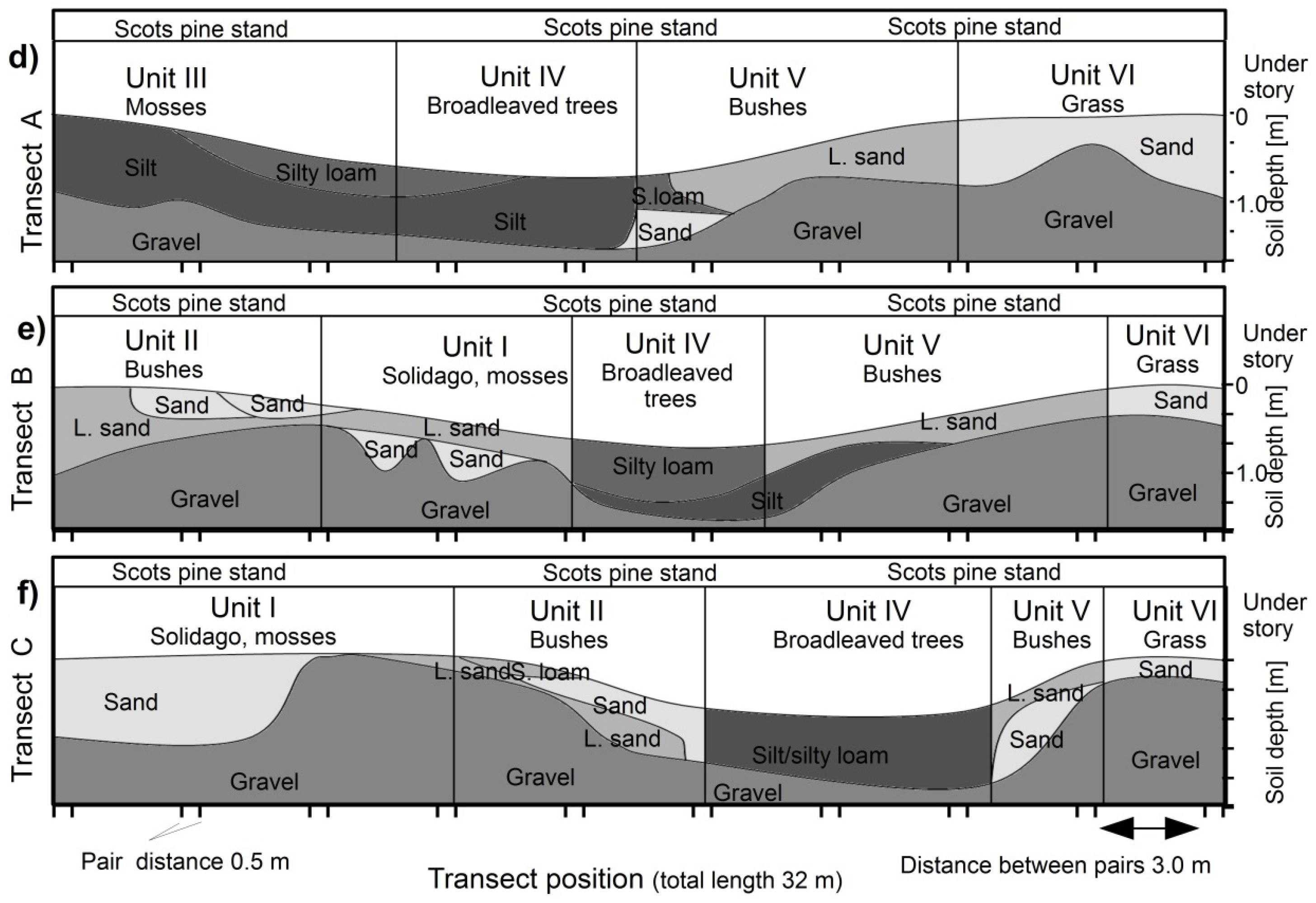
Measurements were carried out in a planted 50 year old Scots pine stand (Pinus sylvestris L.) next to the Hartheim forest meteorological experimental site. The site is located in the Upper Rhine Valley (South-West Germany) about one kilometer east of the Rhine River (47°56′ N, 7°36′ E, 201 m above sea level). The mean annual temperature is 10.3 °C and the mean annual precipitation is 642 mm (Holst et al., 2008). The site was regularly flooded until the mid of the 19th century when the River Rhine was corrected. The topography of the site is flat with minor linear depressions (less than 1 m deep) resulting from former courses of creeks in the floodplain. The soil is a Haplic Regosol (calcaric, humic) [29]. Due to the history of alluvial deposition of substrates, the soil texture changes abruptly vertically within the soil profile and horizontally within short distances. There is a Ah horizon of fine sand-silt-or loamy silt of 5–50 cm depth on top of different fractions of sand and gravel at the most locations. While the pine stand was planted in regular rows, the groundcover and understory allows separating the plot in several homogenous vegetation strata, further called Units I–VI.
2.2. Experimental Design
The measurement plot was positioned across a historical creek bed that formed a minor depression (depth < 1 m) in the former floodplain (Figure 1a,b). The plot was homogenously covered by the planted pine trees and covered different types of soil texture, ground cover and understory vegetation (Figure 1d–f). Measurements were conducted along three 32 m long parallel transects 8 m apart that crossed the depression. Measurement points were regularly distributed on transects as pairs 0.5 m apart and 3 m between the pairs; each transect included 20 measurement points in total.
Measurements and sampling were carried out from 8 to 14 December 2015 in stable weather conditions. At all points we conducted measurement of soil gas fluxes and took soil core samples for soil-physical analysis. We sampled the soil profile down to 1 m depth at all points using a soil probe and assessed the soil texture in the field with the finger test [30]. At all sampling points there was a subsurface gravel layer that at some points reached the surface. The typical sound of the soil probe going through gravel allowed the layer to be identified, yet samples of this layer were mostly lost.
2.3. Measurements of Soil Gas Fluxes
Soil-atmosphere gas fluxes were measured using non-steady-state flow-through chambers. The chambers consisted of a PVC collar and a mobile lid with a vent [31]. The collars (diameter 0.17 m, height 0.25 m) were installed the day before the measurement and inserted approximately 3 cm into the soil. The air in the chamber was circulated via tubes to a Greenhouse Gas Analyzer (GGA; version Ultraportable, Los Gatos Research, CA, USA) for CH4 and CO2 measurements and to a Gas Monitor 1416 (Lumasense, Ballerup, Denmark) for N2O and CF4 (see Section 2.4) analysis. Measurement frequency was 0.5 Hz for the GGA, and every 60 s for the Gas Monitor. Water vapour was measured by both devices and stabilized using a dew point controller set to 4 °C. This greatly improved accuracy and precision of the N2O measurements, as confirmed by tests with a laboratory GC.
Chambers were closed for 15–20 min for the flux measurement. Fluxes of CH4 and CO2 were calculated linearly based on the concentration changes over time of the first five and three minutes, respectively (R2 > 0.95). For N2O flux estimation a linear approach over the whole time span of 15–20 min was used since soil-atmosphere fluxes of N2O were negative and low. When no linear trend was observed (p > 0.05) N2O fluxes were set to zero [32]. Flux measurements of N2O with variable water vapour (coefficient of variation > 0.01) were excluded. Linear regressions were calculated with PROC REG in SAS (SAS 9.2, SAS Institute Inc., Cary, NC, USA)
2.4. Measurements of Soil-Gas Diffusion Coefficients
In addition to our measurements of CO2, CH4 and N2O fluxes, we used CF4 as a tracer gas to measure soil gas diffusivity in situ using a modified McIntyre and Philip approach [31]. A total of 1 mL of diluted CF4 was injected into the chamber after closure so that the initial CF4 concentration reached 15–20 µmol mol−1. The decreasing CF4 concentration was measured over time by the Gas Monitor. The functional relationship between soil gas diffusivity and air-filled pore-space allowed the soil gas diffusivity of the topsoil to be derived. We used a transfer function from Maier et al. [33] that was based on top soil samples from the same site. An error function was fit to the decreasing CF4 concentrations to calculate the soil gas diffusion coefficient for CF4 (DSCF4) (PROC NLIN, SAS 9.4, SAS Institute Inc., Cary, NC, USA) [31]. DSCF4 was divided by the diffusion coefficient of CF4 in air (D0CF4) at the given temperature [34] to obtain the relative soil gas diffusion coefficient DSD0−1insitu, which is independent of the gas species and a useful parameter to assess soil aeration. Gas transport in soil is dominated by molecular diffusion. Yet, wind and wind-induced pressure fluctuations can affect soil gas transport as well [33,35,36]. To avoid wind-induced artefacts it is therefore important to measure soil gas diffusivity in situ under calm conditions. It is also important to ensure proper mixing of air in measurement chambers for both in situ and lab measurements, and to restrict the movement of air in the chambers to ta minimum.
After completing chamber measurements, two 200 cm3 core samples (5 cm height) were taken at each measurement point that was covered by the chamber; and the cores included the humus layer and topsoil. In the lab, the field-fresh soil cores were analysed for soil-physical parameters. Air-filled pore-space was determined by vacuum pycnometry. Soil gas diffusivity (DSD0−1lab) was measured using a nonstationary one-chamber method [37] with neon as a tracer gas at starting concentrations of 100–800 µmol mol−1, and were measured using a micro-gas chromatograph (CP2002P, Chrompack, Middelburg, The Netherlands, with a CP-Molsieve-5A column and He as carrier gas). The soil cores were placed on top of a chamber with gas exchange restricted to diffusion through the sample. After injecting neon into the chamber, the decreasing neon concentration over time allowed to determine the soil gas diffusivity. Air permeability was measured with an apparatus as described by Iversen et al. [38] by relating air flow through the sample to the pressure gradient across the sample. The volumetric soil moisture content was determined by thermogravimetry.
2.5. Methanotrophic Activity
Assuming negligible soil CH4 production, fluxes of atmospheric CH4 into the soil are limited by physical transport and methanotrophic activity. Historically, methanotrophic activity has been measured in the lab through incubation experiment with sieved soil [20,39], i.e., in disturbed systems. Methanotrophic activity under natural conditions can be estimated using gas push-pull tests [40] or a combination of chamber measurements of CH4 consumption and diffusivity in the field [21]. We used the approach of von Fischer et al. [21] to calculate methanotrophic activity µ (s−1).
where is the soil-atmosphere methane flux (mol m−2 s−1), the CH4 concentration at the start of the measurement (mol m−3), the soil gas diffusion coefficient of CH4 (m2 s−1), and the air filled porosity (m3 m−3). Methanotrophic activity was calculated twice: (1) Using the soil gas diffusivity measured in situ to calculate the diffusion coefficient of CH4 in the soil by multiplying DSD0−1insitu by D0 of CH4 in free air (0.21 cm2 s−1), and (2) using the mean DSD0−1lab of the two soil cores. These two approaches were used since laboratory and in situ determination of soil gas diffusivity can yield different values and it is unclear which results are more realistic. D0 of CH4 in free air for both approaches was corrected for barometric pressure and air temperature [41].
2.6. Standardization of GHG Fluxes
Since soil gas fluxes can show clear diurnal pattern at this site [13] we included a control chamber that was measured at the beginning , midday and late afternoon each day throughout the campaign. The observed diurnal flux pattern of the control chamber was used to calculate correction factors and standardize the measured fluxes to the time of the start of the campaign. Standardized fluxes (CO2: ) were calculated by dividing the observed flux () by the respective correction factor ():
The CO2 flux of the control chamber showed a stronger dependency on air temperature than on soil temperature. We thus used air temperature to calculate for all CO2 flux measurement similar to the routine described by Darenova et al. [14]:
where Tair is the air temperature (°C), a is the slope, and b the intercept of the linear regression between CO2 flux and air temperature at the control chamber.
The correlation between the CH4 fluxes of the control chamber and soil temperature was weak, but a clear diurnal pattern was still observed. Correction factors for CH4 fluxes were thus calculated based on the observed diurnal cycle and correction factors were interpolated. For N2O some flux measurements of the control chamber showed no linear trend and had to be set to zero or discarded due to measurement quality issues. Since no clear pattern was observed for the control N2O flux, standardization was omitted.
2.7. Statistical Analysis
For the statistical analysis we followed three approaches. (1) To test whether stratification of the plot based on vegetation patterns could be used to optimize the sampling design, we focused on flux differences between Unit I–VI. (2) To focus on the soil-vegetation effect, we merged Unit I–VI into the category Shoulder (Unit I + VI), Bottom (Unit III + IV), and Transition (Unit II + V) according to their similarities in soil texture, vegetation and topography. (3) To focus on the texture effect separately, all locations were classified individually according to the dominant texture into Sand or Silt. Locations with high gravel content or coarse woody debris were separately classified as Disturbed.
To test differences in mean GHG fluxes between the vegetation strata (Unit I–VI) we used a t-test for normally distributed data and a Mann-Whitney-U test for non-normally distributed data. We used the coefficient of variation (CV) as a measure of variability and uncertainty of the mean estimated soil-atmosphere gas fluxes. To evaluate the un-stratified and the stratified approaches in a simple way we calculated the CV for both approaches [14]. For the stratified approach the weighted mean of the CV of the strata was taken into account according to the sample size of each stratum. Correlations between variables was evaluated using Pearson’s correlation coefficient r for normally distributed data and Spearman’s rank correlation coefficient rs for non-normally distributed variables using PROC CORR (SAS 9.2, SAS Institute Inc., Cary, NC, USA). Significance was set to p < 0.05 for all procedures.
To identify the effect of both continuous (e.g., DSD0−1lab) and categorical variables (texture categories, vegetation units) on response variables (,) we used Random Forest [42]. Random Forest is a tree based ensemble learning method that is now widely used in ecology and also in soil sciences to analyse complex dataset and to derive pedo-transfer functions [43,44]. We used the R package randomForest to build the model [45]. Prior to model building, all continuous variables were standardised and the strength of collinearity between the predictors was assessed. From predictor pairs with a Pearson’s correlation coefficient > 0.5, the predictor variable contributing less to the final model was excluded [46]. To avoid oversaturation of the model, the number of trees to grow in the forest was set to 2000, the number of randomly selected predictor variables at each node was set to 3, and the minimal number of observations at the terminal nodes of the trees were set to 5 [43,44]. Five-fold cross-validation was performed to assess the prediction quality of the model. The coefficient of determination (R2) and the root mean squared error (RMSE) were calculated accordingly.
Based on the Random Forest we built Generalized Mixed Models, with vegetation category or texture class as nominal categories (PROC GLM, SAS 9.2, SAS Institute Inc., Cary, NC, USA). Vegetation unit and texture class were positively correlated and consequently one or the other was used to build a model. The final model was built up by stepwise reducing AIC (Akaike information criterion) that was chosen to account for small sampling size.
3. Results and Discussion
3.1. Standardization of Temporal Variability of Greenhouse-Gas Fluxes
The soil at the Hartheim site was a source of CO2 and sink for CH4 and N2O at all measurement times and points despite top soil moisture conditions being near saturation due to several rain events before the campaign. During the campaign there was fog and dew, meaning soil moisture was stable at 12% vol. at 0.3 m depth (permanently installed monitoring probe) and 25% in the topsoil (mean of 120 soil core samples). Mean soil temperature at 1 cm depth was 6.0 °C during the campaign and ranged from 5.3 to 7.1 °C. Mean air temperature was 5.0 °C, and ranged from 1.0 °C to 10.3 °C. Wind conditions were calm.
Repeated measurements of the CO2 flux at the control chamber showed a strong correlation (R2 = 0.83) with air temperature (Figure 2a) that was reflected in the measurement throughout the spatial replicates (Figure 2a, grey x-symbols). The estimated slope (Equation (3), a = 0.68 µmol m−2 s−1 °C−1) and intercept (b = 0.15 µmol m−2 s−1) of this linear regression were used to standardize measured CO2 fluxes to temperature at the starting time of the campaign. Measured CO2 fluxes were 0.52–2.51 µmol m−2 s−1 and temperature-derived correction factors for CO2 fluxes were 0.8–2.1 (Figure 2b, solid line). Standardizing of CO2 fluxes (Equation (2)) resulted in a slightly smaller range of flux values (0.52–2.42 µmol m−2 s−1).
Repeated measurements of the CH4 flux at the control chamber were not significantly correlated with air temperature, but slow changes over time were observed (Figure 2b). We calculated correction factors by dividing observed fluxes at the control chamber by the CH4 flux at the starting time of the campaign. The CH4 flux correction factor was then interpolated between measurements of the control chamber. The correction factor for CH4 fluxes were 0.7–1.1 (Figure 2e, solid line), meaning the standardization effect for CH4 fluxes was much weaker compared to CO2 fluxes.
Out of the total 62 N2O flux measurements, 6 measurements failed due to problems with the water vapour conditioning and 18 measurements were set to zero flux. Nitrous oxide flux was always negative, i.e., N2O was consumed by the soil, and N2O fluxes were much lower than CH4 fluxes (Figure 2c,f). Consequently, N2O flux measurements were not standardized due to an insufficient number of high-quality, non-zero flux measurements at the control chamber (Figure 2c).
The observed CO2 fluxes agree well with the fluxes known from monitoring campaigns at this site [13,37]. The observed mean CH4 flux of −2.39 nmol s−1 m−2 is at the higher end of uptake measurements according to Smith et al. [18], which would be expected for the well aerated forest soil at Hartheim. The observed mean N2O flux of −0.05 nmol s−1 m−2 is within the range of values listed by Chapuis-Lardy et al. [11], where N2O fluxes as negative as −3.1 nmol m−2 s were reported. Since soil temperature above 5 °C are considered to favour N2O consumption by soils, even higher N2O uptake can be expected at our site in warmer periods of the year [47,48].
3.2. Spatial Variability of Soil Gas Fluxes
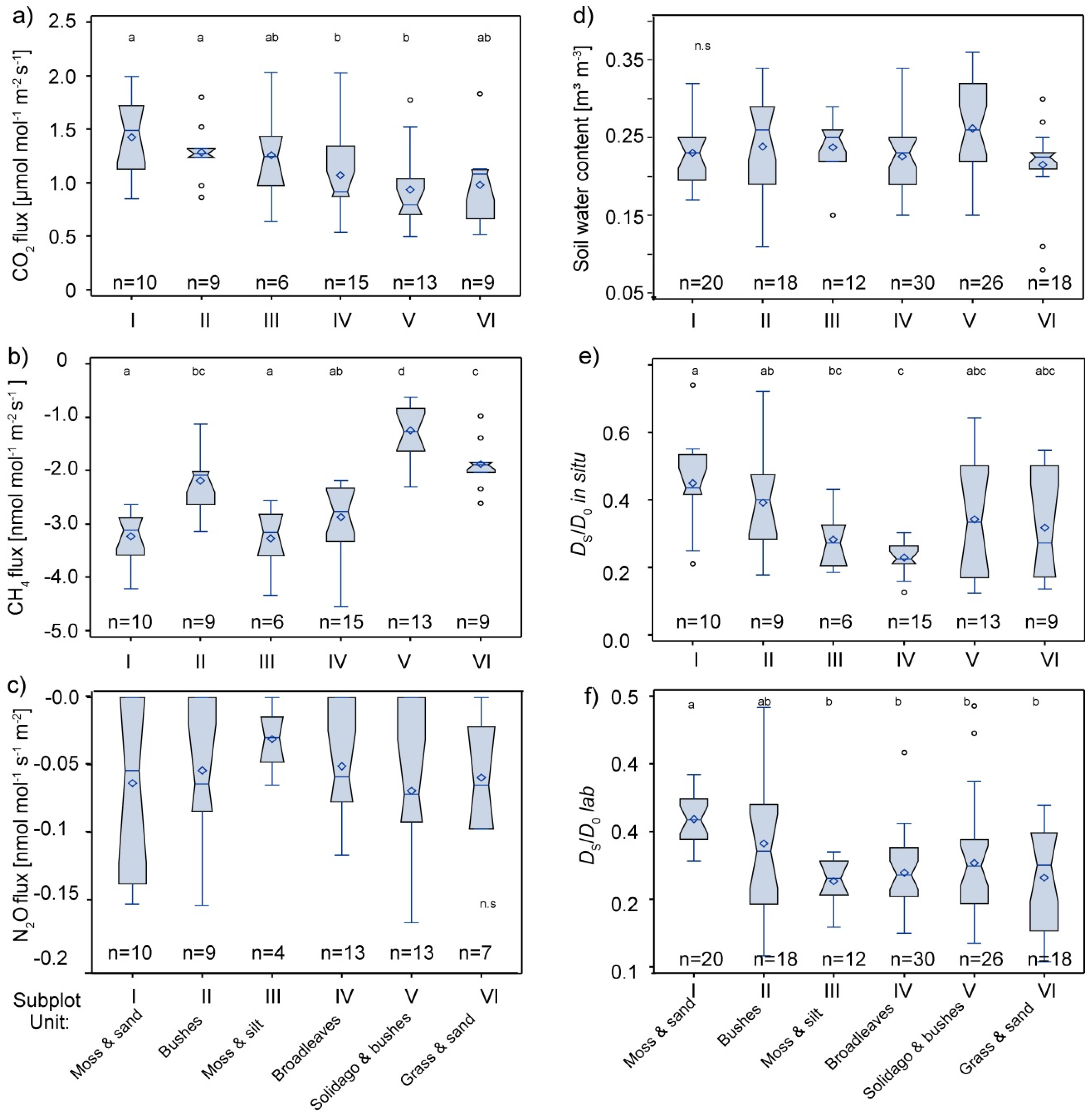
CH4 fluxes between Unit I–VI differed substantially (Table 2, Figure 3b). Lower but significant differences were observed in CO2 fluxes (Figure 3a). N2O fluxes of the different strata were not significantly different, which is probably due to the high number of zero-flux measurements in all strata (Figure 3c). The highest CH4 consumption was observed in the two silt strata (Unit III & IV) and the southern shoulder of the depression (Unit I, sand/gravel; Figure 3b).
Considering the entire un-stratified plot, spatial variability (evaluated as coefficient of variation CV) of the standardized CO2 and CH4 fluxes and non-standardized N2O flux was highest for N2O and similar for CO2 and CH4 (Table 2) and agrees well with data from literature [14,49]. Since the vegetation strata could explain some of the spatial variability of the soil gas fluxes at our site, our stratification approach reduced the CV for CH4 substantially, from 38% to 24% (Table 2); however, it was less effective for CO2 and had almost no effect for N2O.
The RandomForest model showed that the vegetation units contributed substantially to the explanation of the spatial variability of the CO2 flux and especially of the CH4 flux. Total porosity, air filled pore-space, relative soil gas diffusivity and air permeability were highly correlated with one another. Therefore, only relative soil gas diffusivity was used in the final model. Vegetation unit was also highly correlated with soil texture class, so that the latter was excluded from the final model.
For the CH4 flux, the ranking of Variable Importance in the RF model revealed vegetation unit, CO2 Flux and soil water content to be the most relevant explanatory variables. Mean decrease of accuracy in prediction on the Out of bag samples (%IncMSE) when excluded from the model were 75%, 32%, and 13%. The decrease in Node impurity was 25, 11, and 5. The coefficient of determination was found to be 0.95 on the original dataset. R2 was found to be 0.57–0.81 with 5-fold cross-validation. RMSE varied between 19% to 34% of the mean flux. Thus, the selected variables generally are useful to explain the CH4 flux, but predictive accuracy is limited.
The RandomForest model showed that CO2 flux could be best explained by CH4 flux, relative soil gas diffusivity and vegetation unit. Relative importance was much lower and independent variables within the ranking were less unequivocal for the CO2 flux with %IncMSE values of 26%, 20% and 19%. Decrease in Node impurity was 14, 13, and 10. Although the coefficient of determination of the original data was 0.91, cross-validation results showed much less predictive accuracy with 0.06–0.66 R2. RMSE was also poor with 53% to 95% of mean flux.
Stratification approaches have been successfully applied using topographical elements like ditches and fields [50], hill-slope position [51], and plant communities [52]. Few studies though could stratify or explain spatial variability of GHG fluxes on the plot scale. Shvaleva et al. [49] showed that tree cover had an effect on net N2O fluxes and that CH4 fluxes were affected by soil organic carbon content. Darenova et al. [14] identified litter thickness and local soil moisture as important factors affecting CO2 fluxes on the plots scale within a forest and grassland. We did not observe such effects, yet we identified the vegetation strata as important factor affecting CO2 and CH4 fluxes. Since soil texture and vegetation were strongly correlated at our site, it is not possible disentangling the two factors. Nevertheless, stratifying the plot by dominant understory vegetation helped to reduce the uncertainty in the estimated mean CO2 and CH4 flux stemming from spatial variability. Thus, sampling designs for monitoring GHG at this site could be optimized by stratifying the site into different vegetation units, and distributing equally sampling locations within each unit.
Studies comparing plots of different vegetation could show that tree species can affect CH4 consumptions by soils [25,26,49,53,54]. Menyailo et al. [26] observed that tree species had an effect on methanotrophic activity in an afforestation, but that the composition of high affinity methantrophs was not altered. Borken & Beese [25] attributed the observed differences in CH4 uptake between forest sites to the different litter quality and soil moisture. Similar as to our site, Borken & Beese [25] observed no effect of vegetation on N2O fluxes. Niklaus et al. [55] observed that CH4 uptake and soil N2O emissions decreased with plant species richness in a grassland experiment. They attributed the decrease in CH4 uptake to an increase in soil water content. In contrast, Unit I with moss cover had significantly higher CH4 uptake than Unit VI with grass cover, while both have similar water content, soil texture and diffusivity (Figure 3d–f). This could indicate a direct effect of the vegetation on CH4 uptake, with either species of higher succession (grasses) inhibiting CH4 uptake, or species of lower succession (mosses) enhancing CH4 uptake, as known from peatlands [56,57]. Understanding which dynamic is occurring merits further investigation.
3.3. Interaction of Soil Physical Parameters, Soil Gas Fluxes, and Soil-Vegetation Units
Air-filled pores-space, soil gas diffusivity and air permeability of the soil core samples correlated well with each other (Pearson’s r > 0.7). Lab measurements of soil gas diffusivity (DSD0−1lab) correlated well with in situ measurements (DSD0−1insitu) (r: 0.59), while DSD0−1insitu yielded larger values (0.12–0.74) than DSD0−1lab (0.11–0.49) (Figure 3e,f). This was also observed in previous studies [21,31] and can be attributed to uncertainties in the methods and different reference volumes between laboratory and field chambers. Soil gas diffusivity in Unit I was significantly higher than in the other units according to both methods, and both vegetation units with silt (Units III & IV) had low diffusivity values and less variability.
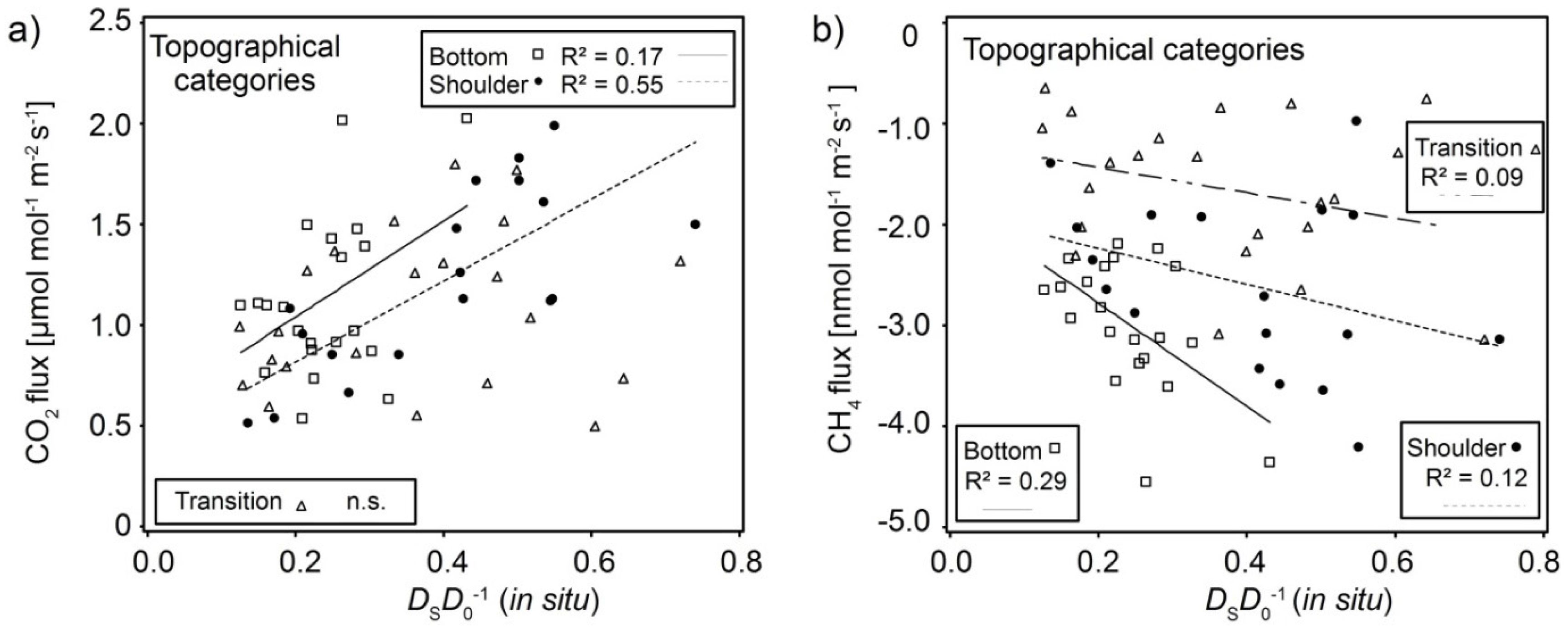
For further analysis we used merged topographical categories Shoulder (Unit I + VI), Bottom (Unit III + IV), and Transition (Unit II + V). Soil texture and aggregation was substantially different between the topographical categories. We observed similar relationships between fluxes and soil-physical parameters (Figure 4), albeit shifted between categories. Correlations were generally less pronounced for the Transition category, since different textures and conditions were merged. As N2O fluxes could not be standardized, no further analysis of the data was performed.
Standardized CO2 fluxes showed a strong correlation with DSD0−1insitu in sand-dominated Shoulder category and a weak correlation in the silt-dominated Bottom category (Figure 4a). Soil CO2 fluxes result from soil respiration and these correlations can be interpreted as an indicator of activity of roots and other soil biota. Such activity supports and maintains soil structure and thereby soil gas diffusivity through increased aggregation and pore formation. As aggregates in sandy soil are more fragile and strongly dependent on roots, CO2 fluxes and soil gas diffusivity would be more dependent on one another in the sandy category compared to the silty category.
Standardized CH4 consumption increased with increasing DSD0−1insitu in all categories (Figure 4b). Although the CH4 consumption in the Shoulder category (Figure 3b, Unit I) was as high as in Bottom category (Figure 3b, Unit III & IV), a stronger correlation between soil gas diffusivity and CH4 consumption could be observed in silty Bottom category. CH4 consumption was highest in the Bottom category at any given DSD0−1insitu compared to the other categories.
The increase in CH4 consumption with soil gas diffusivity is known from numerous studies [5,18,24,58,59], and is often addressed as an effect of water-filled pore-space, or rather air-filled pore-space. High-affinity methanotrophic microbes are ubiquitous in aerated soil and specifically seem to live on the surface of aggregates and pores [54,55] that facilitate access to CH4. The rate of CH4 consumption is consequently limited, amongst other factors, by the supply of atmospheric CH4. This supply is controlled by the rate of gas transport into the soil and generally dominated by the molecular diffusion [18]. In another study, Guckland et al. [59] found that the annual uptake rates of atmospheric CH4 in three forest stands was affected by the clay content. They attributed their results to either higher soil gas diffusivity, since the clay content affects the soil structure, or higher methanotrophic activity.
3.4. Interaction of CH4 Fluxes and Methanotrophic Activity with Soil Respiration
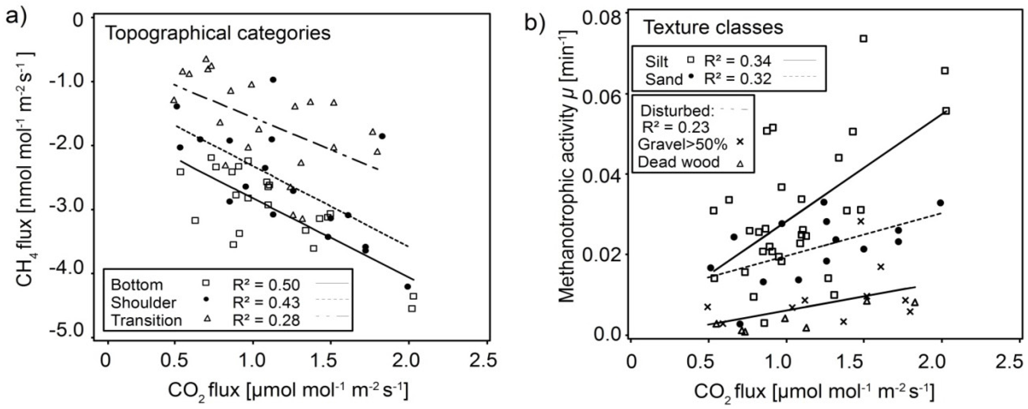
Standardized CH4 fluxes correlated well with standardized CO2 fluxes only when separated into the different topographical categories (Figure 5a) and texture classes (not shown). Specifically, CH4 consumption increased with soil respiration in all three topographical categories. A generalized linear model using the topographical category (n = 3) as independent nominal category and the CO2 flux and the interaction of CO2 flux and topographical category as independent variable could explain 62% of the variability in CH4 flux (R2 = 0.62). The model was improved by adding interactions between soil gas diffusivity (DSD0−1insitu) and topographical category (R2 = 0.68).
The correlation between CH4 consumption and CO2 flux was stronger than the correlation between CH4 consumption and soil gas diffusivity (Figure 4b and Figure 5a). Therefore, in addition to the increased diffusivity and thus aeration that favours both CH4 consumption and soil respiration (Figure 4a), high-affinity methanotrophs may profit when occupying habitats in the vicinity of sources of soil CO2. Warner et al. [28], who studied the spatial and temporal variability in soil gas fluxes on the plot scale, also found a positive correlation between CH4 consumption and CO2 fluxes (personal communication). Dubey et al., (2000) [60] likewise found larger populations of methanotrophs and higher CH4 oxidation activity in the rhizosphere than in bulk soil samples from dryland rice fields. Consequently, those findings in combination with our correlations suggest that sampling locations at our site with more roots (and thus relatively more rhizosphere) have both higher soil respiration and higher CH4 consumption despite differences in plant physiology and physico-chemical soil properties. Additionally the parallel CH4-CO2 flux relationships from different topographical categories with the different dominant soil textures (Figure 5a) reflect a range of habitat qualities for methanotrophic microbes.
To further focus on the effect of soil texture and possible methanotroph habitats, the dataset was classified into the following soil texture classes: Sand, Silt, and Disturbed (a special class containing dead woody debris or gravel content > 50%). Methanotrophic activity µ (Equqtion (1)) [21] was positively correlated with soil CO2 flux in all classes (Figure 4d) with the highest activity in Silt followed by Sand and lastly Disturbed locations. Additionally, µ increased the most with soil CO2 flux in Silt. This last result agrees with the positive correlation between CH4 consumption and soil respiration. It also further supports the idea that high-affinity methanotrophs profit when occupying habitats in the vicinity of sources of soil CO2 through multiple dynamics. First, this could result from more stable habitat conditions due to aggregate formation and more stable aggregates in Silt since high-affinity methanotrophs are affected by physical disturbance [61]. Second, methanotrophs would benefit from “hidden” production of CH4 in anoxic cores of soil aggregates [6]. Such microsite methanogenesis may improve with both increased aggregate size and higher carbon availability within aggregates [62]. Third, a major fraction of soil respiration originates from the rhizosphere and belowground litter as microbial heterotrophic respiration, including methylotrophic microbes [63]. Increasing soil respiration would mean increasing heterotrophic respiration, methylotrophy, and, thus, methanotrophy.
The low methanotrophic activity measured at the Disturbed locations probably results from two effects. Since gravel has less surface area, the high gravel content (Figure 4d) at some of the locations would result in a smaller pore surface area in comparison to silt and sand locations. As methantrophs live preferably on soil-pore surfaces (i.e., aggregate edges) [64], this means the is less suitable pore surface available at locations with high gravel content. A lab analysis revealed that dead woody debris was a weak source of CH4 (not shown), which is known from other studies [28]. At Disturbed locations with dead woody debris (DWD) near the surface we expect therefor that the methane consumption in the mineral soil was partly offset by methane emissions of the DWD, and that the real methanotrophic activity is therefor higher than that what we observed.
In summary, our results suggest that silty soil with its larger pore surface area and greater aggregate size and stability represents a better habitat for methanotrophs. Furthermore, improved methanotrophic activity and consequently CH4 consumption were correlated with increasing soil respiration, suggesting mutualistic interactions between cohabitating heterotrophs and methylotrophs. This supports the idea of the rhizosphere as preferred habitat for methanotrophs. If so, these results provide evidence that greater quantities microbial hotspots as associated with rhizospheres and aggregate surfaces have a noticeable effect on plot-scale variability of greenhouse gas fluxes, specifically for CH4. We strongly suggest further studies on this topic include molecular quantification of the functional genes (pmoA and mmoX) specific for methanotrophs, to better investigate the preferred habitats of high-affinity methantrophs.
4. Conclusions
Proper standardization is necessary to disentangle temporal and spatial variability of soil gas fluxes as CO2 and CH4 fluxes experience substantially different diurnal variation which would mask relationships between the fluxes. We conclude that CH4 consumption at our site was substantially different between vegetation units and soil textures. Within similar vegetation units or soil textural classes, the spatial variability of CH4 consumption depended not only on gas diffusivity, but also on soil respiration that reflects the soil biological activity. We attribute the observed differences between the texture classes to different qualities of habitat for methanotrophic microbes with more habitable surface in Silt than in Sand. As most soil respiration originates from the rhizosphere and belowground litter, our observations indicate that the rhizosphere and belowground litter, facilitates directly or indirectly a preferred living space for methantrophs.
Acknowledgments
We would like to thank our colleagues from the Chair of Mereology for the support and access to their experimental site, Dennis Wheeler for his help in the field and lab, and Karl Stahr for the training course in field methods. This research was supported by the German Research Foundation (DFG, Ma-5826/2-1).
Author Contributions
M.M. conceived and designed the experiments; M.M., C.N. and S.P. performed the experiments and analyzed the data, M.M., K.S. and P.N. wrote the paper.
Conflicts of Interest
The authors declare no conflict of interest. The funding sponsors had no role in the design of the study; in the collection, analyses, or interpretation of data; in the writing of the manuscript, and in the decision to publish the results.
References
- Hartmann, D.L.; Klein Tank, A.M.G.; Rusticucci, M.; Alexander, L.V.; Brönnimann, S.; Charabi, Y.; Dentener, F.J.; Dlugokencky, E.J.; Easterling, D.R.; Kaplan, A.; et al. Observations: Atmosphere and Surface. In Climate Change 2013. The Physical Science Basis; Working Group I contribution to the Fifth Assessment Report of the Intergovernmental Panel on Climate Change; Stocker, T.F., Ed.; Cambridge University Press: Cambridge, UK; New York, NY, USA, 2014. [Google Scholar]
- Ryan, M.G.; Law, B.E. Interpreting, measuring, and modeling soil respiration. Biogeochemistry 2005, 73, 3–27. [Google Scholar] [CrossRef]
- Forster, P.; Ramaswamy, V.; Artaxo, P.; Berntsen, T.; Betts, R.; Fahey, D.W.; Haywood, J.; Lean, J.; Lowe, D.C.; Myhre, G.; et al. Changes in Atmospheric Constituents and in Radiative Forcing. In Climate Change 2007: The Physical Science Basis; Solomon, S., Ed.; Cambridge University Press: Cambridge, UK; New York, NY, USA, 2007. [Google Scholar]
- Conrad, R. Soil Microorganisms as Controllers of Atmospheric Trace Gases (H2, CO, CH4, OCS, N2O, and NO). Microbiol. Rev. 1996, 60, 609–640. [Google Scholar] [PubMed]
- Smith, K.A.; Ball, T.; Conen, F.; Dobbie, K.E.; Massheder, J.; Rey, A. Exchange of greenhouse gases between soil and atmosphere: Interactions of soil physical factors and biological processes. Eur. J. Soil Sci. 2003, 54, 779–791. [Google Scholar] [CrossRef]
- Kuzyakov, Y.; Blagodatskaya, E. Microbial hotspots and hot moments in soil: Concept & review. Soil Biol. Biochem. 2015, 83, 184–199. [Google Scholar] [CrossRef]
- Le Mer, J.; Roger, P. Production, oxidation, emission and consumption of methane by soils: A review. Eur. J. Soil Biol. 2001, 37, 25–50. [Google Scholar] [CrossRef]
- Hanson, R.S.; Hanson, T.E. Methanotrophic bacteria. Microbiol. Rev. 1996, 60, 439–471. [Google Scholar] [PubMed]
- Dunfield, P.F. The soil methane sink. In Greenhouse Gas Sinks; Reay, D.S., Hewitt, C.N., Smith, K.A., Grace, J., Eds.; CABI: Wallingford, UK, 2007; pp. 152–170. [Google Scholar]
- Davidson, E.A.; Verchot, L.V. Testing a conceptual model of soil emissions of nitrous and nitric oxides. Glob. Biogeochem. Cycles 2000, 14, 1035–1043. [Google Scholar] [CrossRef]
- Chapuis-Lardy, L.; Wrage, N.; Metay, A.; Chotte, J.-L.; Bernoux, M. Soils, a sink for N2O? A review. Glob. Chang. Biol. 2007, 13, 1–17. [Google Scholar] [CrossRef]
- Davidson, E.A.; Belk, E.; Boone, R.D. Soil water content and temperature as independent or confounded factors controlling soil respiration in a temperate mixed hardwood forest. Glob. Chang. Biol. 1998, 4, 217–227. [Google Scholar] [CrossRef]
- Maier, M.; Schack-Kirchner, H.; Hildebrand, E.E.; Schindler, D. Soil CO2 efflux vs. soil respiration: Implications for flux models. Agric. For. Meteorol. 2011, 151, 1723–1730. [Google Scholar] [CrossRef]
- Darenova, E.; Pavelka, M.; Macalkova, L. Spatial heterogeneity of CO2 efflux and optimization of the number of measurement positions. Eur. J. Soil Biol. 2016, 75, 123–134. [Google Scholar] [CrossRef]
- Dalal, R.C.; Allen, D.E.; Livesley, S.J.; Richards, G. Magnitude and biophysical regulators of methane emission and consumption in the Australian agricultural, forest, and submerged landscapes: A review. Plant Soil 2008, 309, 43–76. [Google Scholar] [CrossRef]
- Davidson, E.A.; Ishida, F.Y.; Nepstad, D.C. Effects of an experimental drought on soil emissions of carbon dioxide, methane, nitrous oxide, and nitric oxide in a moist tropical forest. Glob. Chang. Biol. 2004, 10, 718–730. [Google Scholar] [CrossRef]
- Striegl, R.G.; McConnaughey, T.A.; Thorstenson, D.C.; Weeks, E.P.; Woodward, J.C. Consumption of atmospheric methane by desert soils. Nature 1992, 357, 145–147. [Google Scholar] [CrossRef]
- Smith, K.A.; Dobbie, K.E.; Ball, B.; Bakken, L.R.; Sitaula, B.K.; Hansen, S.; Brumme, R.; Borken, W.; Christensen, S.; Priemé, A.; et al. Oxidation of atmospheric methane in Northern European soils, comparison with other ecosystems, and uncertainties in the global terrestrial sink. Glob. Chang. Biol. 2000, 6, 791–803. [Google Scholar] [CrossRef]
- Fest, B.; Hinko-Najera, N.; von Fischer, J.C.; Livesley, S.J.; Arndt, S.K. Soil Methane Uptake Increases under Continuous Throughfall Reduction in a Temperate Evergreen, Broadleaved Eucalypt Forest. Ecosystems 2016, 20, 368–379. [Google Scholar] [CrossRef]
- Bender, M.; Conrad, R. Kinetics of CH4 oxidation in oxic soils exposed to ambient air or high CH4 mixing ratios. FEMS Microbiol. Lett. 1992, 101, 261–270. [Google Scholar] [CrossRef]
- Von Fischer, J.C.; Butters, G.; Duchateau, P.C.; Thelwell, R.J.; Siller, R. In situ measures of methanotroph activity in upland soils: A reaction-diffusion model and field observation of water stress. J. Geophys. Res. 2009, 114. [Google Scholar] [CrossRef]
- Wolf, B.; Chen, W.; Brüggemann, N.; Zheng, X.; Pumpanen, J.; Butterbach-Bahl, K. Applicability of the soil gradient method for estimating soil-atmosphere CO2, CH4, and N2O fluxes for steppe soils in Inner Mongolia. J. Plant Nutr. Soil Sci. 2011, 174, 359–372. [Google Scholar] [CrossRef]
- Flechard, C.; Neftel, A.; Jocher, M.; Amann, C.; Fuhrer, J. Bi-directional soil/atmosphere N2O exchange over two mown grassland systems with contrasting management practices. Glob. Chang. Biol. 2005, 11, 2114–2127. [Google Scholar] [CrossRef]
- Ball, B.; Smith, K.A.; Klemedtsson, L.; Brumme, R.; Sitaula, B.K.; Hansen, S.; Priemé, A.; MacDonald, J.; Horgan, G.W. The influence of soil gas transport properties on methane oxidation in a selection of northern European soils. J. Geophys. Res. 1997, 102, 23309. [Google Scholar] [CrossRef]
- Borken, W.; Beese, F. Methane and nitrous oxide fluxes of soils in pure and mixed stands of European beech and Norway spruce. Eur. J. Soil Sci. 2006, 57, 617–625. [Google Scholar] [CrossRef]
- Menyailo, O.V.; Abraham, W.-R.; Conrad, R. Tree species affect atmospheric CH4 oxidation without altering community composition of soil methanotrophs. Soil Biol. Biochem. 2010, 42, 101–107. [Google Scholar] [CrossRef]
- Nauer, P.A.; Dam, B.; Liesack, W.; Zeyer, J.; Schroth, M.H. Activity and diversity of methane-oxidizing bacteria in glacier forefields on siliceous and calcareous bedrock. Biogeosciences 2012, 9, 2259–2274. [Google Scholar] [CrossRef]
- Warner, D.L.; Villarreal, S.; McWilliams, K.; Inamdar, S.; Vargas, R. Carbon Dioxide and Methane Fluxes From Tree Stems, Coarse Woody Debris, and Soils in an Upland Temperate Forest. Ecosystems 2017. [Google Scholar] [CrossRef]
- WRB. World Reference Base for Soil Resources 2014. International Soil Classification System for Naming Soils and Creating Legends for Soil Maps; FAO: Rome, Italy, 2014. [Google Scholar]
- Ad-hoc-Arbeitsgruppe Boden der Staatlichen Geologischen Dienste und der Bundesanstalt für Geowissenschaften und Rohstoffe; Bundesanstalt für Geowissenschaften und Rohstoffe. Bodenkundliche Kartieranleitung; Auflage: 5; E. Schweizerbart’sche Verlagsbuchhandlung: Stuttgart, German, 2005. [Google Scholar]
- Schack-Kirchner, H.; Gaertig, T.; Wilpert, K.V.; Hildebrand, E.E. A modified McIntyre and Phillip approach to measure top-soil gas diffusivity in-situ. J. Plant Nutr. Soil Sci. 2001, 164, 253–258. [Google Scholar] [CrossRef]
- De Klein, C.; Harvey, M. Nitrous Oxide Chamber Methodology Guidelines. Available online: http://globalresearchalliance.org/wp-content/uploads/2015/11/Chamber_Methodology_Guidelines_Final-V1.1-2015.pdf (accessed on 17 November 2016).
- Maier, M.; Schack-Kirchner, H.; Aubinet, M.; Goffin, S.; Longdoz, B.; Parent, F. Turbulence effect on gas transport in three contrasting forest soils. Soil Sci. Soc. Am. J. 2012, 76, 1518–1528. [Google Scholar] [CrossRef]
- Raw, C.; Raw, T.T. Diffusion of gaseous fluoromethanes in air. Chem. Phys. Lett. 1976, 44, 255–256. [Google Scholar] [CrossRef]
- Redeker, K.R.; Baird, A.J.; Teh, Y.A. Quantifying wind and pressure effects on trace gas fluxes across the soil–atmosphere interface. Biogeosciences 2015, 12, 7423–7434. [Google Scholar] [CrossRef]
- Laemmel, T.; Mohr, M.; Schack-Kirchner, H.; Schindler, D.; Maier, M. Direct observation of wind-induced pressure-pumping on gas transport in soils. Soil Sci. Soc. Am. J. 2017. [Google Scholar] [CrossRef]
- Maier, M.; Schack-Kirchner, H.; Hildebrand, E.E.; Holst, J. Pore-space CO2 dynamics in a deep, well-aerated soil. Eur. J. Soil Sci. 2010, 61, 877–887. [Google Scholar] [CrossRef]
- Iversen, B.V.; Schjønning, P.; Poulsen, T.G.; Moldrup, P. In situ, on-site and laboratory measurements of soil air permeability. Soil Sci. 2001, 166, 97–106. [Google Scholar] [CrossRef]
- Gulledge, J.; Schimel, J.P. Moisture control over atmospheric CH4 consumption and CO2 production in diverse Alaskan soils. Soil Biol. Biochem. 1998, 30, 1127–1132. [Google Scholar] [CrossRef]
- Nauer, P.A.; Schroth, M.H. In Situ Quantification of Atmospheric Methane Oxidation in Near-Surface Soils. Vadose Zone J. 2010, 9, 1052. [Google Scholar] [CrossRef]
- Fuller, E.N.; Schettler, P.D.; Giddings, J.C. New method for prediction of binarz gas/phase diffusion coefficients. Ind. Eng. Chem. 1966, 58, 18–27. [Google Scholar] [CrossRef]
- Hastie, T.; Tibshirani, R.; Friedman, J.H. The Elements of Statistical Learning. Data Mining, Inference, and Prediction, 2nd ed.; Springer: New York, NY, USA, 2016. [Google Scholar]
- Cutler, D.R.; Edwards, T.C.; Beard, K.H.; Cutler, A.; Hess, K.T.; Gibson, J.; Lawler, J.J. Random Forests for classification in ecology. Ecology 2007, 88, 2783–2792. [Google Scholar] [CrossRef] [PubMed]
- Were, K.; Bui, D.T.; Dick, Ø.B.; Singh, B.R. A comparative assessment of support vector regression, artificial neural networks, and random forests for predicting and mapping soil organic carbon stocks across an Afromontane landscape. Ecol. Indic. 2015, 52, 394–403. [Google Scholar] [CrossRef]
- Liaw, A.; Wiener, M. Classification and Regression by randomForest. R News 2002, 2, 18–22. [Google Scholar]
- Dormann, C.F.; Elith, J.; Bacher, S.; Buchmann, C.; Carl, G.; Carré, G.; Marquéz, J.R.G.; Gruber, B.; Lafourcade, B.; Leitão, P.J.; et al. Collinearity: A review of methods to deal with it and a simulation study evaluating their performance. Ecography 2013, 36, 27–46. [Google Scholar] [CrossRef]
- Glatzel, S.; Stahr, K. Methane and nitrous oxide exchange in differently fertilised grassland in southern Germany. Plant Soil 2001, 231, 21–35. [Google Scholar] [CrossRef]
- Ryden, J.C. N2O exchange between a grassland soil and the atmosphere. Nature 1981, 292, 235–237. [Google Scholar] [CrossRef]
- Shvaleva, A.; Siljanen, H.M.P.; Correia, A.; Costa E Silva, F.; Lamprecht, R.E.; Lobo-do-Vale, R.; Bicho, C.; Fangueiro, D.; Anderson, M.; Pereira, J.S.; et al. Environmental and microbial factors influencing methane and nitrous oxide fluxes in Mediterranean cork oak woodlands: Trees make a difference. Front. Microbiol. 2015, 6, 1104. [Google Scholar] [CrossRef] [PubMed]
- Schrier-Uijl, A.P.; Kroon, P.S.; Leffelaar, P.A.; van Huissteden, J.C.; Berendse, F.; Veenendaal, E.M. Methane emissions in two drained peat agro-ecosystems with high and low agricultural intensity. Plant Soil 2010, 329, 509–520. [Google Scholar] [CrossRef]
- Konda, R.; Ohta, S.; Ishizuka, S.; Arai, S.; Ansori, S.; Tanaka, N.; Hardjon, O.A. Spatial structures of N2O, CO2, and CH4 fluxes from Acacia mangium plantation soils during a relatively dry season in Indonesia. Soil Biol. Biochem. 2008, 40, 3021–3030. [Google Scholar] [CrossRef]
- West, A.E.; Brooks, P.D.; Fisk, M.C.; Smith, L.K.; Holland, E.A.; Jaeger, I.C.; Babcock, S.; Lai, R.S.; Schmidt, S.K. Landscape patterns of CH4 fluxes in an alpine tundra ecosystem. Biogeochemistry 1999, 45, 243–264. [Google Scholar] [CrossRef]
- Reay, D.; NedwellL, D.; McNamara, N.; Ineson, P. Effect of tree species on methane and ammonium oxidation capacity in forest soils. Soil Biol. Biochem. 2005, 37, 719–730. [Google Scholar] [CrossRef]
- Hiltbrunner, D.; Zimmermann, S.; Karbin, S.; Hagedorn, F.; Niklaus, P.A. Increasing soil methane sink along a 120-year afforestation chronosequence is driven by soil moisture. Glob. Chang. Biol. 2012, 18, 3664–3671. [Google Scholar] [CrossRef]
- Niklaus, P.A.; Le Roux, X.; Poly, F.; Buchmann, N.; Scherer-Lorenzen, M.; Weigelt, A.; Barnard, R.L. Plant species diversity affects soil-atmosphere fluxes of methane and nitrous oxide. Oecologia 2016, 181, 919–930. [Google Scholar] [CrossRef] [PubMed]
- Raghoebarsing, A.A.; Smolders, A.J.P.; Schmid, M.C.; Rijpstra, W.I.C.; Wolters-Arts, M.; Derksen, J.; Jetten, M.S.M.; Schouten, S.; Sinninghe Damste, J.S.; Lamers, L.P.M.; et al. Methanotrophic symbionts provide carbon for photosynthesis in peat bogs. Nature 2005, 436, 1153–1156. [Google Scholar] [CrossRef] [PubMed]
- Putkinen, A.; Larmola, T.; Tuomivirta, T.; Siljanen, H.M.P.; Bodrossy, L.; Tuittila, E.-S.; Fritze, H. Peatland succession induces a shift in the community composition of Sphagnum-associated active methanotrophs. FEMS Microbiol. Ecol. 2014, 88, 596–611. [Google Scholar] [CrossRef] [PubMed]
- Brumme, R.; Borken, W. Site variation in methane oxidation as affected by atmospheric deposition and type of temperate forest ecosystem. Glob. Biogeochem. Cycles 1999, 13, 493–501. [Google Scholar] [CrossRef]
- Guckland, A.; Flessa, H.; Prenzel, J. Controls of temporal and spatial variability of methane uptake in soils of a temperate deciduous forest with different abundance of European beech (Fagus sylvatica L.). Soil Biol. Biochem. 2009, 41, 1659–1667. [Google Scholar] [CrossRef]
- Dubey, S.K.; Sinha, A.S.; Singh, J.S. Spatial variation in the capacity of soil for CH4 uptake and population size of methane oxidizing bacteria in dryland rice agriculture. Curr. Sci. 2000, 78, 617–620. [Google Scholar]
- Roslev, P.; Iversen, N.; Henriksen, K. Oxidation and assimilation of atmospheric methane by soil methane oxidizers. Appl. Environ. Microbiol. 1997, 63, 874–880. [Google Scholar] [PubMed]
- Ebrahimi, A.; Or, D. Hydration and diffusion processes shape microbial community organization and function in model soil aggregates. Water Resour. Res. 2015, 51, 9804–9827. [Google Scholar] [CrossRef]
- Butterfield, C.N.; Li, Z.; Andeer, P.F.; Spaulding, S.; Thomas, B.C.; Singh, A.; Hettich, R.L.; Suttle, K.B.; Probst, A.J.; Tringe, S.G.; et al. Proteogenomic analyses indicate bacterial methylotrophy and archaeal heterotrophy are prevalent below the grass root zone. PeerJ 2016, 4, e2687. [Google Scholar] [CrossRef] [PubMed]
- Stiehl-Braun, P.A.; Powlson, D.S.; Poulton, P.R.; Niklaus, P.A. Effects of N fertilizers and liming on the micro-scale distribution of soil methane assimilation in the long-term Park Grass experiment at Rothamsted. Soil Biol. Biochem. 2011, 43, 1034–1041. [Google Scholar] [CrossRef]
Figure 1.
(a) Topographical map of the Hartheim experimental site based on last-pulse laser scan data; (b) Position of the sampling transects on the topographical map; (c) Sampling plot divided into understory vegetation strata; (d–f) Catenae along Transect A–C including the respective vegetation strata.


Figure 2.
Greenhouse gas fluxes measured in the control chambers (black) and spatial replicates (grey) for (a) CO2, (b) CH4, and (c) N2O, and in the spatial replicates for (d) CO2, (e) CH4, and (f) N2O. For CO2, the correlation between air temperature and CO2 fluxes in the control chamber (dashed line in (a)) was used to calculate correction factors (solid lines in (b)) and standardized CO2 fluxes (circles) from measured CO2 fluxes (triangles). For CH4, correlation with air temperature was weak; interpolated CH4 fluxes in the control chamber (dashed lines in (c)) were used directly to calculate correction factors (solid lines in (d)) and standardized CH4 fluxes (circles) from measured CH4 fluxes (triangles) for the respective date and time. Standardization of N2O fluxes was not possible due to insufficient number of quality measurements in the control chamber (e). Hence, measured N2O fluxes were used for downstream analysis.

Figure 3.
Boxplots of standardized soil-atmosphere gas fluxes of (a) CO2 and (b) CH4, (c) non-standardized N2O fluxes, (d) soil water content, (e) soil gas diffusivity measured in situ (DSD0−1 in situ), and (f) soil gas diffusivity measured in the laboratory (DSD0−1lab) of the different subplot units. The mean value is indicated by the rhomb and the horizontal lines indicate the 25th 50th and 75th percentile. Signficant differences in the mean value are indicated by a different letter above.

Figure 4.
(a) Standardized CO2 fluxes increase with increasing DSD0−1insitu for the Bottom and Shoulder category; (b) Standardized CH4 consumption increases with increasing DSD0−1insitu.
Figure 4.
(a) Standardized CO2 fluxes increase with increasing DSD0−1insitu for the Bottom and Shoulder category; (b) Standardized CH4 consumption increases with increasing DSD0−1insitu.

Figure 5.
(a) Standardized CH4 consumption increases with increasing CO2 fluxes within the respective topographical categories; (b) Methanotrophic activity (Equation (1)) increases with increasing CO2 within the respective texture classes, with the strongest increase in silt. R2 represent the coefficient of determination.


Table 1.
Vegetation units used to stratify the sampling plot.
| Unit | Topography | Understory & Ground Vegetation | Soil Texture |
|---|---|---|---|
| Unit I | Southern shoulder & plain | Solidago gigantea (L.) and moss species | Sand & gravel to loamy sand |
| Unit II | Southern slope | Bushes, Ligustrum vulgare (L.); Crataegus monogyna (Jacq.) | Sandy gravel to sandy loam |
| Unit III | Bottom-slope | Mosses (e.g., Scleropodium purum, L.) | Silt and silty loam. |
| Unit IV | Bottom | 10–20 year old broadleaves Juglans regia (L.), Tilia platyphyllos (L.), Carpinus betulus (L.), less groundcover | Silt and silty loam. |
| Unit V | Norther slope & shoulder | Bushes, Ligustrum vulgare (L.); Crataegus monogyna (Jacq.) | Sandy gravel to sandy loam |
| Unit VI | Northern plain | (few) Solidago gigantea (L.), grass species | Sand and gravel |
Table 2.
Mean flux and coefficient of variation (CV) of GHG for all measurement or as weighted sum of all strata.
Table 2.
Mean flux and coefficient of variation (CV) of GHG for all measurement or as weighted sum of all strata.
| Flux | All Measurements | Weighted Sum of Strata | ||
|---|---|---|---|---|
| Mean | CV | Mean | CV | |
| CO2 (µmol s−1 m−2) | 1.13 | 36% | 1.13 | 33% |
| CH4 (nmol s−1 m−2) | −2.39 | 38% | −2.39 | 24% |
| N2O (nmol s−1 m−2) | −0.05 | 88% | −0.05 | 87% |
© 2017 by the authors. Licensee MDPI, Basel, Switzerland. This article is an open access article distributed under the terms and conditions of the Creative Commons Attribution (CC BY) license (http://creativecommons.org/licenses/by/4.0/).
Share and Cite
MDPI and ACS Style
Maier, M.; Paulus, S.; Nicolai, C.; Stutz, K.P.; Nauer, P.A. Drivers of Plot-Scale Variability of CH4 Consumption in a Well-Aerated Pine Forest Soil. Forests 2017, 8, 193. https://doi.org/10.3390/f8060193
AMA Style
Maier M, Paulus S, Nicolai C, Stutz KP, Nauer PA. Drivers of Plot-Scale Variability of CH4 Consumption in a Well-Aerated Pine Forest Soil. Forests. 2017; 8(6):193. https://doi.org/10.3390/f8060193
Chicago/Turabian StyleMaier, Martin, Sinikka Paulus, Clara Nicolai, Kenton P. Stutz, and Philipp A. Nauer. 2017. "Drivers of Plot-Scale Variability of CH4 Consumption in a Well-Aerated Pine Forest Soil" Forests 8, no. 6: 193. https://doi.org/10.3390/f8060193
Note that from the first issue of 2016, this journal uses article numbers instead of page numbers. See further details here.