A New Soil Moisture Downscaling Approach for SMAP, SMOS, and ASCAT by Predicting Sub-Grid Variability


1
Forschungszentrum Jülich, Institute of Bio- and Geosciences: Agrosphere (IBG-3), 52428 Jülich, Germany
2
Instituto Hispano Luso de Investigaciones Agrarias, University of Salamanca, 37185 Salamanca, Spain
*
Author to whom correspondence should be addressed.
Remote Sens. 2018, 10(3), 427; https://doi.org/10.3390/rs10030427
Submission received: 12 January 2018
/
Revised: 27 February 2018
/
Accepted: 8 March 2018
/
Published: 9 March 2018
(This article belongs to the Special Issue Retrieval, Validation and Application of Satellite Soil Moisture Data)
Abstract
:Several studies currently strive to improve the spatial resolution of coarse scale high temporal resolution global soil moisture products of SMOS, SMAP, and ASCAT. Soil texture heterogeneity is known to be one of the main sources of soil moisture spatial variability. With the recent development of high resolution maps of basic soil properties such as soil texture and bulk density, relevant information to estimate soil moisture variability within a satellite product grid cell is available. We use this information for the prediction of the sub-grid soil moisture variability for each SMOS, SMAP, and ASCAT grid cell. The approach is based on a method that predicts the soil moisture standard deviation as a function of the mean soil moisture based on soil texture information. It is a closed-form expression using stochastic analysis of 1D unsaturated gravitational flow in an infinitely long vertical profile based on the Mualem-van Genuchten model and first-order Taylor expansions. We provide a look-up table that indicates the soil moisture standard deviation for any given soil moisture mean, available at https://doi.org/10.1594/PANGAEA.878889. The resulting data set helps identify adequate regions to validate coarse scale soil moisture products by providing a measure of representativeness of small-scale measurements for the coarse grid cell. Moreover, it contains important information for downscaling coarse soil moisture observations of the SMOS, SMAP, and ASCAT missions. In this study, we present a simple application of the estimated sub-grid soil moisture heterogeneity scaling down SMAP soil moisture to 1 km resolution. Validation results in the TERENO and REMEDHUS soil moisture monitoring networks in Germany and Spain, respectively, indicate a similar or slightly improved accuracy for downscaled and original SMAP soil moisture in the time domain for the year 2016, but with a much higher spatial resolution.

1. Introduction
Soil moisture is an important driver for the control of weather and climate feedbacks [1]. The scientific community has well recognized the very important role of soil moisture in Earth science applications, and innovative approaches and techniques for monitoring, modelling, and using soil moisture data have been developed [2]. Global observations of soil moisture are available from several spaceborne sensors, such as the Soil Moisture Ocean Salinity (SMOS) [3], the Soil Moisture Active Passive (SMAP) [4], and the Advanced Scatterometer (ASCAT) [5] missions. However, the spatial scale of these mission data is several tens of kilometers, which is too coarse for a large variety of applications, especially when referring to the emerging hyper-resolution modelling trend [6,7] that requires more highly resolved observations of critical hydrological variables. However, that is a demand we currently seem ill-prepared to meet [8].
Recently, several reviews investigated different aspects related to soil moisture observation [2,9,10,11,12,13], as well as soil moisture downscaling [14]. The main challenge is the very high spatio-temporal variability of soil moisture [15,16,17,18]. In the last 40 years, a large number of studies have attempted to understand the spatial and temporal variability of soil moisture from the local to the global scale [12,19,20]. Indeed, several researchers carried out detailed studies in different environmental and climatic settings to assess soil moisture variability. Since the description of the soil moisture variance as a function of the observation scale by a power law decay by Rodriguez-Iturbe et al. [21], different methods have been applied [22,23], including statistical [24,25,26] and geostatistical approaches [27,28,29,30], temporal stability analysis [31,32,33], and wavelet techniques [34,35,36,37,38]. Important to mention is the study by Famiglietti et al. [15], who analyzed more than 36,000 soil moisture measurements in the central US. In addition to a fractal scaling rule, they found that soil moisture standard deviation versus mean moisture in this humid climate exhibited a convex-upward relationship, i.e., that the standard deviation increases until mean soil moisture reaches around 0.2 m3 m−3 and then decreases beyond that. Further studies also found a steadily increasing behavior for other regions with modifications regarding soil, climate, and vegetation [39,40,41,42,43,44]. However, Vereecken et al. [45] explained the general shape of the soil moisture standard deviation versus mean moisture as a function of hydraulic parameter variation.
According to Salvucci [46], as well as Lawrence and Hornberger [47], the origin of soil moisture heterogeneity can be found in meteorology [48,49], vegetation characteristics [39], and groundwater [41], as well as landscape attributes such as topography [50] and soil texture [51]. Not fully explored is the vegetation-soil moisture variability relationship [52,53]. In arid and semiarid regions, vegetation strongly influences soil moisture temporal variation immediately after a rain event due to interception, but also later due to different solar irradiance and resulting soil evaporation. However, these differences become less pronounced as mean annual precipitation increases [54]. The spatial variability of soil moisture is therefore related to the spatial heterogeneity of vegetation. However, Teuling and Troch [55] showed that the main discriminating factor between increasing or decreasing spatial variance of soil moisture with soil moisture mean is whether or not the soil dries below the critical moisture content that defines the transition between unstressed and stressed transpiration. To a large extent, this depends on the soil texture. Similarly, Riley and Shen [44] found that the reduction in soil moisture variance with increasing mean past a particular intermediate value of the mean depends on the magnitude of evapotranspiration due to partial water stress limitation. In addition, Clapp et al. [56] found that approximately 75% of the standard deviation of soil moisture measured at the field scale could be accounted for by analyzing soil texture. Gwak and Kim [51] showed that soil texture was a dominant factor in soil moisture distribution, and Crow et al. [57] indicated that soil texture is a dominant physical control of soil moisture at finer scales. Additionally, Wang et al. [58] indicate that soil texture plays an important role in soil moisture variability, where vegetation dampens the relationship between the mean and standard deviation of soil moisture. Vereecken et al. [45] demonstrated that the shape of the soil moisture variance over mean curve can be explained to a large extent by the spatial variance of soil hydraulic properties, indicating that soil texture is an important driver of soil moisture spatio-temporal variability. Here, in the scientific community, the general perception exists that the shape of the soil moisture variance over mean curve has to be convex, with lower variance at the dry and wet end of the curve and higher variance at intermediate conditions. Some soil moisture observations support this view, whilst others show steadily increasing soil moisture variance with mean soil moisture (see examples in Qu et al. [59]). Vereecken et al. [45] elaborated on the shape of the respective curves as a result of soil texture with the conclusion that the peak at intermediate mean soil moisture occurs for finer textured soils only. They related the curves to Brooks and Corey hydraulic parameters and found that convex shapes occur only with dominant variance in the soil pore distribution index (i.e., the Brooks and Corey parameter β). It is important to note that a dominant variability in the air entry value (α), in saturated hydraulic conductivity (lnKs), or in the vertical correlation length of the Brooks-Corey parameters would lead to a steady decrease in soil moisture variability from wet to dry mean soil moisture conditions.
Thus far, a global higher resolution (~1 km) soil moisture product from SAR sensors has not been made available [2], and the disaggregation of coarse resolution products remains the focus [60,61,62,63]. Validation activities for SMAP [64,65,66,67,68,69], SMOS [65,70,71,72,73,74], and ASCAT [5,73,75] generally found good agreement with in situ measurements. Therefore, current research strives to increase the spatio-temporal resolution of these products by auxiliary data. With thermal infrared data from multispectral satellites, a downscaling to 100 m has been achieved, exploiting the ratio of actual to potential evaporation [76]. Similarly, machine learning methods have been used to downscale SMOS by MODIS land surface temperature [77]. Verhoest et al. [78] used a copula-based probability distribution function that reflects the expected distribution function of modelled soil moisture for a given SMOS observation for downscaling. The combined use of observations from active and passive satellite microwave instruments in a soil moisture data assimilation system with a spatially distributed 3D ensemble Kalman filter have been shown to improve soil moisture results [79]. Driven by the SMAP concept [80] and the launch of the Sentinel-1 satellites [81], downscaling by radar gains importance [82]. Recently, a first combined SMAP-Sentinel-1 product has been made available at a 3 km resolution, and 1 km resolution data is available for scientific analysis [83]. The downscaling already on the brightness temperature level by backscatter is based on time series statistical analysis of the radar-radiometer data relationships [84,85], but can also be forward calculated based on physical approaches [86]. All these methods identify proxy data for downscaling and need to statistically estimate the magnitude of the disaggregation, but they neglect soil texture as an important information source for the sub-grid variability of soil moisture.
Qu et al. [59] developed a method to predict sub-grid variability of soil moisture based on basic soil data, such as texture. They derived a closed-form expression to describe how soil moisture variability depends on mean soil moisture () using stochastic analysis of 1D unsaturated gravitational flow based on the Mualem-van Genuchten (MvG) model. The method has already been proven to reliably predict soil moisture variability of small catchments [59]. Qu et al. [59] showed that their method is able to predict convex functions and that this specific relationship is related to the variability of the MvG parameter n. In recent times, high resolution data on soil properties for the whole globe has become increasingly available [87,88], e.g., the SoilGrids data sets at a 1 km [89] and 250 m [90] resolution, respectively. By combining the method of Qu et al. [59] and the SoilGrids data set [89], the variance over mean soil moisture relationship can be predicted for each grid of coarse scale soil satellite data products. In this study, we adapt this method to be used on global scale soil moisture products such as those of SMAP, SMOS, and ASCAT. To this end, a look-up table was developed that indicates the sub-grid soil moisture standard deviation as a function of soil moisture. This information can be used for downscaling coarse resolution soil moisture products. As an example, we scaled the SMAP soil moisture data product from its original resolution down to 1 km resolution by using field capacity as a proxy for soil moisture heterogeneity. The results were validated using two in situ soil moisture networks in Germany and Spain for the year 2016.
2. Soil Data Base and Moisture Variability Estimation Methods
The general procedure of the method proposed here is based on the SoilGrids data set, which is transferred to hydraulic parameters for the MvG model of unsaturated gravitational water flow. After identifying the high resolution pixels of the hydraulic parameters comprised in each coarse satellite grid cell, we related the covariance of soil water content and pressure head to the variance and covariance of MvG parameters based on the method by Qu et al. [59].
2.1. A Closed Form Expression to Estimate Soil Moisture Variability
The basis for this method proposed by Qu et al. [59] forms the MvG model that describes the water retention curve given by:
where
and the hydraulic conductivity curve given by:
In the water retention function, is the pressure head (cm), is the effective saturation (-), (cm3 cm−3) is the saturated water content, (cm3 cm−3) is the residual water content, and (cm3 cm−3) is the actual soil moisture. (cm−1), (-), and (-) () are shape parameters. The hydraulic conductivity function is directly related to the water retention function by , where is the saturated hydraulic conductivity (cm d−1) and (cm d−1) is the hydraulic conductivity. is the pore connectivity parameter.
The method proposed by Qu et al. [59] is based on the approach of Zhang et al. [91], who developed a first-order stochastic model for gravity-dominated flow in second-order stationary media. In this respect, a second-order stationary stochastic process is either a linear process or a non-linear process that can be transformed to a linear process by subtracting a deterministic component. Second order stationarity means that spatial heterogeneity can be fully described by the first two moments of a Gaussian distribution: the mean and the variance. Stationarity refers to the fact that the mean does not show a spatial trend (at each location, the expected mean is identical). The main idea is to explain the relationship as a function of the mean and standard deviation of the soil hydraulic parameters. The decomposition of the stochastic process into mean and perturbations of the parameters and variables can be performed by an infinite sum of terms, but here it is approximated by a finite number of terms of its Taylor series. By keeping the first-order terms only, Qu et al. [59] derived a relationship that expresses the standard deviation of soil water content as a function of the standard deviation in MvG model parameters. More specifically, they related the covariance of soil moisture and pressure head to the variance and covariance of MvG parameters (, , , and ) using Equations (1) and (3) to derive the following closed-form expression describing the relationship:
is the log-transformed saturated hydraulic conductivity () used here for mathematical convenience. is the vertical correlation length of the respective parameters. The coefficients – and – contain the mean of the parameters:
For more details about the derivation, we refer to the supplementary information given by Qu et al. [59]. Both Qu et al. [59] and Toth et al. [92] assume to be 0.5 [93]. Please note that Qu et al. [59] assumed to be constant, but here we calculate the spatial average of for each grid cell (). To describe the full function, we employed the pressure head vector . In order to transform into , we used the following equation:
Note that the relationship between and changes for every individual grid cell. Therefore, we provide a global map of including a pixel-based look-up table for specific . A linear interpolation from high accuracy with several digits after the decimal point to was performed. The final results are provided in the same dimensions as the original soil moisture satellite products, i.e., the results for SMAP and SMOS are generated on 406 × 964 and 584 × 1388 grids, respectively. As the ASCAT product is provided as time series data, the sub-grid soil moisture variability is made available in table form where the location can be identified by the ASCAT grid point index.
2.2. SoilGrids
Publicly available soil profile data, such as that of the US National Cooperative Soil Survey Soil Characterization database (NCSS), of the Land Use/Cover Area frame Statistical Survey LUCAS [94], and of the Soil and Terrain Database (SOTER) [95], in addition to further national soil databases, provide the basis for the SoilGrids data set. Additional proxy information, e.g., the Shuttle Radar Topography Mission (SRTM) digital elevation model and Moderate-Resolution Imaging Spectroradiometer (MODIS) satellite imagery, were used to derive highly resolved spatial patterns of soil properties. These covariates were converted to principle components in order to reduce noise and artefacts. The automated mapping procedure makes use of three general methods, i.e., multiple linear regression for predicting pH, texture (%), and bulk density (kg m−3), general linear models with a log-link function for predicting cation exchange capacity (cmol+ kg−1) and organic carbon content (g kg−1), and zero-inflated models for predicting coarse soil fragments (%) and depth to bedrock (cm). Each soil depth is modelled using a separate model that includes different combinations of covariates, resulting in soil properties at seven predefined depths (0, 5, 15, 30, 60, 100, and 200 cm). For the study at hand, we used the top soil layer (0 cm), which provides the largest contribution to a microwave signal recorded by SMAP, SMOS, and ASCAT. Additionally, we decided to use the SoilGrids data base at a 1 km resolution instead of the higher resolution data base at 250 m, because recent studies have shown a trend for satellite product disaggregation towards 1 km grids [65]. It should be noted that SoilGrids is stored in a World Geodetic System 84 (WGS84) regular grid with a 1 km resolution at the equator, i.e., the resolution at other latitudes is higher.
2.3. Toth Pedotransfer Function for MvG Model Parameterization
In order to provide MvG parameters from soil information of SoilGrids, we used the pedotransfer function by Toth et al. [92]. The advantage of this parametric pedotransfer function is that it is based on a continental scale soil data base, the European Hydropedological Data Inventory (EU-HYDI, a successor of the HYPRES data base [96]), rather than a national data base [97,98]. In addition, Toth et al. [92] provide a large variety of model approaches for different input parameters. However, other pedotransfer functions for the MvG model could be applied in a similar way.
In more detail, a linear regression based on pH, clay, silt, and cation exchange capacity, as well as information about top soil or subsoil vertical location, is established for predicting in their model 17, where has been log-transformed before (). Model 21 of their supplement is used for the moisture retention curve parameters, where a regression tree predicts residual water content by fraction, and linear regressions predict from texture and bulk density, from texture, bulk organic carbon content, and top soil or subsoil location, and from the same predictors. and were log-transformed prior to prediction ( and ).
For each individual SoilGrids pixel, the pedotransfer function was applied, and therefore the initial retention parameter maps have the same spatial extent as the original SoilGrids data base. Thus, in the WGS84 projection, no data is available farther South than 62°S.
2.4. Satellite Soil Moisture Data Products
The aim of this study is to predict the sub-grid soil moisture variability of SMOS, SMAP, and ASCAT, the main systems providing global soil moisture records. To this end, the widely used higher level SMAP L3 Radiometer Global Daily 36 km product [99], the CATDS SMOS L3 Global Daily ~25 km product [100], and the ASCAT H110 12.5 km product [5] have been used. The original SMOS and SMAP data grids were resampled to the global, cylindrical Equal-Area Scalable Earth Grid, Version 2.0 (EASE 2.0). This implies that the maximum number of fine pixels from the SoilGrids data base changes from equator to the poles. The number of pixels used to calculate the soil moisture mean and standard deviation will be provided with the final data set. Moreover, the H109 or H110 ASCAT product grid distributed by the EUMETSAT Satellite Application Facility on Support to Operational Hydrology and Water Management (H-SAF) with 12.5 km basic sampling has been used. For this dataset, the maximum number of fine resolution pixels per coarse grid cell also changes from the equator to the poles. The maximum number of fine pixels per coarse grid cell can be reduced by water pixels, which are excluded by the algorithm. The spatial link of fine grid pixels to coarse grid IDs has been identified within ArcGIS.
2.5. How to Use the Estimated Sub-Grid Soil Moisture Variability Data for Downscaling?
In addition to the general investigation of sub-grid heterogeneity for identifying adequate (homogeneous) validation sites and evaluating the representativeness of single soil moisture sensors for large areas covered by a satellite pixel, the estimated function in the final data set can be used for soil moisture disaggregation using proxy information which describes the spatial patterns within each coarse scale satellite pixel. Proxy data can be higher resolution Earth observation data with a proven relationship to soil moisture variability such as surface temperature [101,102], vegetation [103], a combination of both [104], radar backscatter [84], or even soil texture [105]. The proxy data need to be normalized for each individual grid cell. By multiplication with the provided soil moisture standard deviation at the given mean soil moisture, a disaggregation can be performed:
where is the proxy data at fine scale sub-grid y-location and x-location , is the mean of the proxy, and is the standard deviation of the proxy. This means that we disaggregate by the standard score (also called z-scores or normal scores) of the proxy multiplied with . is the predicted soil moisture at this fine scale location. Note that the resolution of the fine scale proxy data should be similar to the soil data set used to estimate . In order to present the principle of the downscaling method, the SMAP soil moisture is downscaled by using a soil field capacity (FC) map as the proxy, which is taken as a representation of the variability of basic soil properties calculated by Equations (1) and (2) with (pF 2.5).
Validation of the downscaled products was performed at two soil moisture networks deployed in Germany (Terrestrial Environmental Observatories, TERENO; Rur catchment) and Spain (Soil Moisture Measurement Stations Network of the University of Salamanca, REMEDHUS). In both regions, several soil moisture validation studies were conducted before [61,65,66,70,73,74,82,106,107]. The Rur catchment comprises a heterogeneous landscape with a hilly high precipitation region covered by forest and grassland in the South, and with flat relatively dryer agricultural dominated loess region in the North [82,108,109]. The general heterogeneity also includes the soil texture [110,111,112]. Within the TERENO observatory, several field-scale wireless soil moisture sensor networks and cosmic ray neutron probes were installed [113,114,115]. Here, we use time domain reflectometry (TDR) sensors at a 5 cm depth at four locations for validation, namely Gevenich, Merzenhausen, Ruraue, and Schoneseiffen. The REMEDHUS network includes 22 stations equipped with Hydra probes (Stevens® Water Monitoring System, Inc., Portland, OR, USA) that measure hourly soil moisture in the top 5 cm of the soil. The land use of the REMEDHUS region is mainly rainfed cereals, fallow, vineyard, and forest-pasture. Opposed to the TERENO observatory, the REMEDHUS area is a relatively homogeneous area in terms of topography. The variability in soil characteristics is somewhat lower compared to the TERENO area [107]. Those different site characteristics make them ideal to test the downscaling algorithm.
In order to evaluate the ability of the different products to capture spatial patterns of the reference dataset (TERENO and REMEDHUS), Pearson´s correlation coefficient is computed between the original SMAP, as well as the two downscaled SMAP products with the reference data yielding one correlation value per day. This method described by Kolassa et al. [116] and already implemented in performance evaluation of multi-scale soil moisture data assimilation [117], suggests using at least ten data points to calculate a spatial correlation at a given time step. Therefore, the robust correlation analysis is performed for the REMEDHUS network only.
3. Results and Discussion
3.1. Specific Analysis Based on Selected Grid Points
We selected four individual pixels to discuss the results in detail, as seen in Figure 1. The selection process of these pixels was driven by the intention to characterize two very different characteristics, i.e., one relatively homogenous and one relatively heterogeneous, respectively, for two regions. First, two coarse scale pixels were selected, located in Germany covering the North of North-Rhine Westphalia (NRW, 51.64°N, 8.40°E) and the North of Rhineland-Palatinate (RLP, 50.30°N, 8.03°E). Similar to the examples in Montzka et al. [118], the first is characterized by soils evolved from Pleistocene morainal plains overlying Jurassic and Triassic rocks (heterogeneous), where the latter soil developed from Devonic sediments as well as fluviatile sediments from the Rhine river system (homogeneous). Then, two coarse scale pixels located in the United States covering central Oregon (OR, 43.72°N, 121.18°W) and South Iowa (IA, 41.06°N, 93.92°W) were selected. The first covers an area where sediments are alternating with volcanic material of different ages (heterogeneous), and the latter is located in the Southern Iowa drift plain covered by loess (homogeneous) [119]. In all regions, the geologic basic material dominates soil evolution towards textural homogeneity or heterogeneity of the coarse pixels.
The clear differentiation in degree of soil textural heterogeneity is visible in Figure 1 for both the US and the German regions. Moreover, the different satellite product grids show large similarities, but the ASCAT grid has a finer resolution, so local heterogeneities in soil texture have a stronger impact on the characteristics. This is especially the case for the relatively homogeneous pixels of RLP and IA. For example, at , is larger than 0.06 for both NRW and OR and all satellite grids, wheras for RLP and IA, SMOS and SMAP show low of less than 0.02 in contrast to ASCAT, with denoting an intermediate soil moisture standard deviation.
By using satellite soil moisture data, the time series of soil moisture standard deviation for each product can be calculated. Figure 2 visualizes the respective time series for the SMAP grids of NRW, RLP, OR, and IA for the year 2016. ASCAT and SMOS time series appear similar. The SMAP mean soil moisture records for the close-by grid cells NRW and RLP are relatively similar with a small offset during the summer period. However, due to the different spatial soil texture heterogeneity, the soil moisture standard deviation is completely different. The heterogeneous NRW grid cell has a with strong temporal dynamics ranging between 0.02 and 0.07, where the RLP grid cell is characterized by stable over time of about 0.015. This is in correspondence to the SMAP functions in Figure 1. For the US grid cells, the differentiation in homogeneous and heterogeneous cells is similar, with a more emphasized difference in the general soil moisture magnitude. That is, soil moisture conditions are generally 0.2 m3 m−3 wetter in IA than in OR. Here, the dryer OR grid cell is characterized by higher soil moisture spatial variability throughout the year than IA. This is in correspondence to the SMAP functions in Figure 1. The very flat curve for IA indicates that Iowa is a suitable target region for coarse scale soil moisture validation studies, which has already been reported and utilized in several studies [120,121,122,123].
3.2. Discussion of Global Heterogeneity Maps
For reasons of brevity, the discussion of the spatial results is performed for the SMAP data set in the following. SMOS and ASCAT show similar patterns of the relationship, but with slightly different absolute values related to the spatial extent of individual pixels. Figure 3 presents the relationship for specific values of ( cm3 cm−3). At , generally low values exist in accordance with the curves in Figure 1, but several regions can already be characterized by elevated . Especially domains in the vicinity of large rivers such as the Nile and Amazon gained diversified texture by the power of large water masses. Similarly, in the Sahel, the climate is the main reason for elevated , because it is a climate region with strong seasonal changes influencing different forms of soil texture development. Volcanic activity and high topography in South East Asia, the Himalaya, and the Andes favor large diversity in soil texture and therefore also elevated . In Northern Europe and Central Canada, where pleistocene morainal plains cover parental rock material, soil development exhibits small-scale texture differences increasing . These general patterns intensify with increasing . The overall patterns of sub-grid soil moisture standard deviation shown in Figure 3 are well-comparable with the results of other methods to identify sub-grid variability, such as the Miller-Miller scaling approach of Montzka et al. [118].
In order to identify the impact of the proposed closed-form expression to describe for satellite data, we calculated the annual mean soil moisture for the year 2016 for the SMAP product. The result is presented in Figure 4a. The overall soil moisture patterns follow the climatic division with very wet soils in the west-continental tropics, very dry conditions in the subtropics, and moderate soil moisture in temperate regions. Using this observed soil moisture as areal mean soil moisture (), the provided look-up table directly outputs the soil moisture standard deviation () for the given grid-cell, shown in Figure 4b. In most regions of the world, soil texture drives soil moisture heterogeneity, but for some regions, a consideration of soil texture variability in soil moisture downscaling is of the utmost importance, visible in the particularly high . For SMAP, these regions are:
- South East Asia
- Amazon basin
- Northern Europe
- Canada
- Qinghai-Tibet Plateau
- Japan, Korea, North East China, South East Russia
- South Chile
The mentioned high textural variability in Sahel results in moderate only, because the annual soil moisture mean is relatively low here. Regions where considering soil texture in SMAP downscaling might be secondary are of course the deserts, but also steppe regions such as (Inner-) Mongolia, Mexico and the US Great Plains, the Northern Brazilian Highlands including the Serras de Borborema and do Espinaco, and the Argentinian Pampas, due to very low soil moisture and/or low textural variability. Therefore, simple resampling of coarse soil moisture observations might be sufficient to receive adequate higher spatial resolution soil moisture maps.
Figure 4c shows the saturated soil moisture or porosity to indicate the wet end at which the maximum soil moisture input gives reasonable estimates. Especially in the tropics for individual points in time, can be larger than due to the different basis data sets so that a reasonable prediction of is not possible.
At the dry end, i.e., in desert regions of Sahara, Arab peninsula, Namib, and central Australia, the SoilGrids data base identified very high sand fractions, which is reasonable. However, as already mentioned, the Toth et al. [92] pedotransfer function uses a constant value of 0.041 for for almost all soil textures (sand fraction larger than 2%). Therefore, the SMAP value for desert soils can be smaller than , precluding the prediction of sub-grid soil moisture standard deviation. This problem can also occur when using other pedotransfer functions providing such as the ones of Schaap et al. [124] and Vereecken et al. [125]. On the other hand, pedotransfer functions assuming or such as Weynants et al. [126] would solve this problem, but at the cost of larger uncertainties for moderate and wet soils. The pedotransfer function of Wösten et al. [96] uses , which can be seen as a compromise and would reduce the problem of unidentified sub-grid soil moisture standard deviation for very dry soil conditions.
3.3. Publication of the Sub-Grid Heterogeneity Product
The final data set is provided in netcdf format at https://doi.org/10.1594/PANGAEA.878889 and contains the information given in Table 1. Latitude, longitude, number of valid pixels, and the mean soil moisture to be matched with the satellite soil moisture observation is given. and are also stored in the data set to identify the valid range of soil moisture for the respective pixel. Because for the SMAP and SMOS soil moisture retrieval different soil texture information has been used than utilized in this study, discrepancies may occur when observations fall outside of the valid range indicated here. We recommend removing these observations from the estimation of sub-grid soil moisture variability, because validity may not be given. For ASCAT, the grid point index and cell number are also provided. Here, , , mean soil moisture, and soil moisture standard deviation are given in cm3 cm−3, although original ASCAT data is provided as the degree of saturation ranging between 0 and 1. A multiplication with the porosity provided with ASCAT data based on NASA´s Land Data Assimilation System [127] or the Harmonized World Soil Database [128] using the Saxton and Rawls [129] pedotransfer function could convert ASCAT data into volumetric units (cm3 cm−3). However, when estimating the soil moisture sub-grid variability for further use, we recommend multiplication with the porosity provided here for consistency reasons.
3.4. Downscaling Results
In order to present and discuss predicted application for downscaling results, we selected the region around the Upper Rhine valley in the Southwest Germany, France, and Switzerland. Figure 5 shows the FC map calculated from surface level soil texture taken from the SoilGrids data base. The low FC values within the Upper Rhine valley clearly differentiate it from the high FC values of organic-rich top soils of the Black Forest, the Vosges, and the German low mountain ranges. This FC map is now used as a proxy for soil moisture downscaling.
Figure 6a shows the soil moisture mean values for 2016 at the original SMAP grid for the region around the Upper Rhine valley. On this very coarse resolution, no real soil moisture patterns can be identified. Figure 6b shows the downscaled soil moisture mean at a 1 km resolution. Neighboring coarse pixels with similar soil moisture appear in similar soil moisture values, but at a high resolution with added sub-grid pattern information, showing the potential of this downscaling by predicting the relationship. However, the different mean soil moisture values of the coarse grid are still clearly visible in the high resolution downscaled soil moisture map, which makes it inadequate for further utilization. Similar patterns also emerge when using other downscaling methods such as that of Das et al. [84], Merlin et al. [76], and Molero et al. [62], in case the spatial discrepancy between coarse and fine resolution is high (e.g., 36 km to ≤ 1 km). Thus, further methods need to be applied in order to balance the sharp edges at the grid border. Here, based on the valid assumption that radiometer footprints follow a Gaussian contribution pattern and the SMAP Level 3 grid is an interpolated result of the raw data, we apply a simple interpolation to graduate soil moisture mean and soil moisture standard deviation between grid centers, i.e.:
Figure 6c shows the downscaled soil moisture based on interpolation (). Here, sharp grid borders are much less pronounced and the remaining edges originate from the proxy normal scores. Now, the soil property pattern is clearly visible in the soil moisture patterns, which is a large improvement compared to the original SMAP data. Larger water bodies such as Lake Constance and other pre-Alpine lakes have a clear impact on soil moisture observations from SMAP as the pixels are generally wetter than surrounding pixels. Here, an adaption of the water mask for the SMAP data processing may help reduce this impact.
Table 2 lists the temporal validation metrics of the original SMAP product compared to the downscaling and downscaled/interpolated results for the sites within the TERENO and REMEDHUS networks. Except for Ruraue, the bias is relatively low for the TERENO stations, and for all sites, the comparison to the products evaluated here results in adequate unbiased root-mean-squared deviation (ubRMSD) and high correlation coefficients (R). There is a small but not always significant trend for improved ubRMSD and R for the downscaled products. For example, for the site Merzenhausen, ubRMSD decreases from 0.043 to 0.037 for the downscaled/interpolated result. Similarly, R increases for that site from 0.803 to 0.817. The results in REMEDHUS confirm the good performance of the downloading procedure. The downscaled product improves or at least maintains the standards of the original SMAP product. However, the differences between the original and the downscaled SMAP are in general less marked than in the TERENO network, probably due to the smaller variability of the texture characteristics in the REMEDHUS area, where the soils are in general very sandy [130] and thus less influenced by the texture-based nature of the downscaling algorithm. As found in similar validation experiments [107], the highest bias and errors occur in H9, owing to the fact that this station is located in a valley area occasionally flooded.
Regarding the validation of spatial patterns, the annual mean correlation coefficient is very similar for the three products in the REMEDHUS region (SMAP original: 0.3204, SMAP downscaled: 0.3331, SMAP downscaled/interpolated: 0.3187), suggesting that their performance capturing the spatial patterns is similar. However, the smaller spatial R in comparison with the temporal one should be noted, as also shown in other studies that used soil moisture data from passive satellites, even in the case of downscaled data products [61,131]. The temporal course of the spatial correlation of the three products for the REMEDHUS network provides interesting insights on the downscaling results, even outdoing the temporal correlation analysis, where no remarkable differences were found for the original SMAP, the downscaled, and the interpolated/downscaled series (Table 2). In the case of the spatial patterns (Figure 7), although the three series follow similar trends, the downscaled/interpolated product showed remarkably higher values at many dates (14 occasions of spatial correlation R > 0.5, compared to two for both SMAP original and SMAP downscaled). Examining the spatial patterns resulting from each method in Figure 6, it can be easily seen that the interpolated map removed the blocky structure both of the original and the downscaled maps, whilst ingesting the sub-grid spatial variability from the soil map. Thus, even in a relatively homogeneous soil area like REMEDHUS, the instantaneous pattern of the 19 stations soil moisture is better captured in many cases.
Generally, at a level of 0.4 during spring, late autumn, and winter, the spatial correlation decreases during summer months for all products. During these very dry conditions with soil moisture below 0.1 m3m−3, the spatial variability of soil moisture is further decreased, thus reducing the correlations. Further implementation of alternative proxies obtained from weather radar networks may support the downscaling procedure. Another explanation is the sampling of SMAP data towards the fixed 36 km grid, whereas the real -3dB radiometer footprint at a 40° incidence angle is an ellipse with a ~40 km mean radius. Both explanations indicate the potential of the recently published 9 km SMAP radiometer data as a basis for downscaling towards a 1 km resolution.
3.5. Validity of the Approach
The first set of results of this study is the sub-grid soil moisture standard deviation maps for SMAP, SMOS, and ASCAT. As the soil moisture standard deviation prediction is fully based on texture information, the accuracy of this first result depends on the accuracy of the SoilGrids1km data set. The ~110,000 soil profiles used to fit global spatial prediction models per soil variable are not evenly distributed over the globe. Very dense sampling is obtained in US, Mexico, and Europe, whereas very sparse information is available for Central Asia, Australia, and North Africa [89]. In dense sampling regions, the model fitting procedure gains high performance, whereas in sparse sampling regions, the fitting might not cover the full soil heterogeneity. Hengl et al. [89] mentioned that their regression models account for ca. 20–50% of observed variability in the target variables. They assume that it is unlikely that any effort to map the distribution of soils at a resolution of 1 km could explain a much larger proportion of the total variation in soil properties, as much of this variation occurs over distances of less than 1 km [39]. This explanation is supported by a higher resolution study that generated SoilGrids250m by the same method, which gained a much higher performance [90]. As stated in the introduction, soil texture can be a dominant feature for soil moisture spatial heterogeneity, but it is not the only one. Further heterogeneity is introduced by the spatial variability of topography, vegetation, land use, and rainfall. Therefore, the presented data of soil moisture sub-grid variability only provides the first insights into the actual heterogeneity of the region. In addition, it has to be noted that the continuous spatial maps of SoilGrids1km have been generated from both soil sample point data and spatially distributed by spatial predictors such as topography from SRTM and vegetation information from MODIS. For example, in SoilGrids1km, the distribution of sand, silt, and clay fractions, i.e., the main contributions to the pedotransfer function, is mainly controlled by the predictors topography and lithology [89]. Therefore, single contributors cannot be disentangled so that in the SoilGrids1km texture information, topography and vegetation information is also implemented.
The second set of results of this study show the exemplified application of the sub-grid soil moisture standard deviation maps for SMAP downscaling towards a 1 km resolution. The validation of the downscaling procedure in Section 3.4 gives a hint on the potential of using the predicted sub-grid soil moisture variability for soil moisture downscaling not only for the SMAP mission, but also for the SMOS and ASCAT mission data. In addition to the issues mentioned earlier in this section, the downscaling proxy needs to show the spatial patterns of soil moisture at the sub-grid scale. FC used in this study for downscaling is a static proxy where the FC normal scores do not vary with time, but the high resolution spatial soil moisture patterns may vary with moisture conditions. Here, applying alternative temporal dynamic proxy data such as backscatter [84] or soil evaporative efficiency [76] could improve the results of this study.
As the presented downscaling approach uses soil moisture estimates with a coarse resolution, a water mask is already applied for SMAP, SMOS, and ASCAT. Therefore, water pixels in the SoilGrids1km data base, indicated with no data (see for example Lake Constance in Figure 6), are neglected and do not contribute to the spatial statistics during downscaling to avoid twofold application. This is in contrast to downscaling algorithms starting at the brightness temperature level, e.g., the SMAP-Sentinel-1 product, where the water mask based on MODIS 250 m data is implemented during the soil moisture retrieval of already downscaled brightness temperature.
4. Conclusions and Outlook
In this study, we adapted the method of Qu et al. [59] about predicting the sub-grid variability of soil moisture for global scale soil moisture product grids of SMAP, SMOS, and ASCAT. The method uses a closed-form expression to describe how soil moisture variability depends on mean soil moisture using stochastic analysis of 1D unsaturated gravitational flow based on the Mualem-van Genuchten (MvG) model. By implementation of high resolution soil properties data provided by SoilGrids at 1 km [89], it is possible to predict the standard deviation over mean soil moisture relationship for each coarse scale grid cell. The final result is a look-up table map that indicates the sub-grid soil moisture standard deviation of a SMAP, SMOS, or ASCAT pixel when providing the coarse grid soil moisture. It is made available at https://doi.org/10.1594/PANGAEA.878889.
Results were analyzed temporally for specific coarse pixels over Germany and US, indicating feasible prediction of the soil moisture standard deviation over mean curves with strong differences between homogeneous and heterogeneous grid cells with respect to basic soil properties. The application for SMAP soil moisture time series for the year 2016 provided the alternating sub-grid soil moisture standard deviation for the respective pixels, which are in good agreement with the SMAP functions. Referring to the US pixels, Iowa is generally wetter than Oregon, but the dryer Oregon grid cell is characterized by higher soil moisture spatial variability throughout the year than Iowa. The latter shows a very low and flat curve, which makes Iowa a perfect target region for coarse scale soil moisture validation. The spatial analysis was performed on a global scale. We discuss the spatial patterns of the standard deviation over mean relationship for specific mean soil moisture values, and additionally for the SMAP mean soil moisture of the year 2016. Due to generally low soil moisture, the sub-grid soil moisture variability is negligible in deserts and steppe regions. In contrast, medium wet regions in the vicinity of large rivers, with strong seasonal climatic variation, pleistocene morainal plains, high volcanic activity, or high topographical dynamics are characterized by high sub-grid soil moisture variability.
The disaggregation of coarse resolution soil moisture products is an important task to enable its usage for regional applications. Several disaggregation methods need information on the scaling magnitude of a disaggregation proxy, i.e., to identify how large the deviation of individual fine pixels from areal mean soil moisture is. This is typically done by time series analysis or specific models. Here, we provide the statistics to disaggregate soil moisture to finer resolutions, where it is possible to provide the soil moisture patterns by surface temperature observations or radar backscatter. In order to illustrate that the predicted sub-grid heterogeneity can be used for soil moisture downscaling, we generated a higher resolution soil moisture data set for SMAP by soil texture as a downscaling proxy. More specifically, the static field capacity information from the SoilGrids data set was used to scale SMAP soil moisture down to a 1 km resolution. Validation results in the TERENO and REMEDHUS networks indicate a similar or slightly improved accuracy for downscaled and original SMAP soil moisture in the time domain, but with a much higher spatial resolution. Applying temporal dynamic proxy data such as microwave backscatter or soil evaporative efficiency could improve the encouraging results. In order to reduce the blocky structure in downscaled SMAP soil moisture data due to the large-scale discrepancy between the 36 km product and the 1 km product, we interpolated the coarse soil moisture prior to downscaling. Here, the use of the 9 km SMAP product might circumvent the need for interpolation, and in addition provides a better spatial performance compared to reference measurements.
Acknowledgments
This study was supported by the Helmholtz-Alliance on “Remote Sensing and Earth System Dynamics” and the BelSPO STEREO III HYDRAS+ project. The SoilGrids data set can be accessed at www.soilgrids.org. Soil moisture data for validation was provided by TERENO (Terrestrial Environmental Observatories). The REMEDHUS data was supported by the Junta de Castilla y Léon (SA007U16) project, the Spanish Ministry of Economy and Competitiveness (ESP2015-67549-C3) project and the European Regional Development Fund (ERDF).
Author Contributions
Carsten Montzka conceived and designed the experiments; Kathrina Rötzer performed a pilot study with the support of Heye R. Bogena and Carsten Montzka. Carsten Montzka did the final calculations. Nilda Sanchez supported the validation activities in the REMEDHUS network. All authors wrote the paper.
Conflicts of Interest
The authors declare no conflict of interest.
References
- McColl, K.A.; Alemohammad, S.H.; Akbar, R.; Konings, A.G.; Yueh, S.; Entekhabi, D. The global distribution and dynamics of surface soil moisture. Nat. Geosci. 2017, 10, 100–104. [Google Scholar] [CrossRef]
- Brocca, L.; Ciabatta, L.; Massari, C.; Camici, S.; Tarpanelli, A. Soil moisture for hydrological applications: Open questions and new opportunities. Water 2017, 9, 140. [Google Scholar] [CrossRef]
- Kerr, Y.H.; Waldteufel, P.; Wigneron, J.P.; Delwart, S.; Cabot, F.; Boutin, J.; Escorihuela, M.J.; Font, J.; Reul, N.; Gruhier, C.; et al. The smos mission: New tool for monitoring key elements of the global water cycle. Proc. IEEE 2010, 98, 666–687. [Google Scholar] [CrossRef] [Green Version]
- Entekhabi, D.; Njoku, E.G.; O’Neill, P.E.; Kellogg, K.H.; Crow, W.T.; Edelstein, W.N.; Entin, J.K.; Goodman, S.D.; Jackson, T.J.; Johnson, J.; et al. The soil moisture active passive (smap) mission. Proc. IEEE 2010, 98, 704–716. [Google Scholar] [CrossRef]
- Wagner, W.; Hahn, S.; Kidd, R.; Melzer, T.; Bartalis, Z.; Hasenauer, S.; Figa-Saldana, J.; de Rosnay, P.; Jann, A.; Schneider, S.; et al. The ascat soil moisture product: A review of its specifications, validation results, and emerging applications. Meteorologische Zeitschrift 2013, 22, 5–33. [Google Scholar] [CrossRef]
- Bierkens, M.F.P.; Bell, V.A.; Burek, P.; Chaney, N.; Condon, L.E.; David, C.H.; de Roo, A.; Doll, P.; Drost, N.; Famiglietti, J.S.; et al. Hyper-resolution global hydrological modelling: What is next? “Everywhere and locally relevant”. Hydrol. Processes 2015, 29, 310–320. [Google Scholar] [CrossRef]
- Wood, E.F.; Roundy, J.K.; Troy, T.J.; van Beek, L.P.H.; Bierkens, M.F.P.; Blyth, E.; de Roo, A.; Doll, P.; Ek, M.; Famiglietti, J.; et al. Hyperresolution global land surface modeling: Meeting a grand challenge for monitoring earth’s terrestrial water. Water Resour. Res. 2011, 47. [Google Scholar] [CrossRef]
- McCabe, M.F.; Rodell, M.; Alsdorf, D.E.; Miralles, D.G.; Uijlenhoet, R.; Wagner, W.; Lucieer, A.; Houborg, R.; Verhoest, N.E.C.; Franz, T.E.; et al. The future of earth observation in hydrology. Hydrol. Earth Syst. Sci. Discuss. 2017, 21, 3879–3914. [Google Scholar] [CrossRef]
- Brocca, L.; Crow, W.T.; Ciabatta, L.; Massari, C.; Rosnay, P.D.; Enenkel, M.; Hahn, S.; Amarnath, G.; Camici, S.; Tarpanelli, A.; et al. A review of the applications of ascat soil moisture products. IEEE J. Sel. Top. Appl. Earth Obs. Remote Sens. 2017, 10, 2285–2306. [Google Scholar] [CrossRef]
- Fang, B.; Lakshmi, V. Soil moisture at watershed scale: Remote sensing techniques. J. Hydrol. 2014, 516, 258–272. [Google Scholar] [CrossRef]
- Ochsner, T.E.; Cosh, M.H.; Cuenca, R.H.; Dorigo, W.A.; Draper, C.S.; Hagimoto, Y.; Kerr, Y.H.; Larson, K.M.; Njoku, E.G.; Small, E.E.; et al. State of the art in large-scale soil moisture monitoring. Soil Sci. Soc. Am. J. 2013, 77, 1888–1919. [Google Scholar] [CrossRef] [Green Version]
- Vereecken, H.; Schnepf, A.; Hopmans, J.W.; Javaux, M.; Or, D.; Roose, D.O.T.; Vanderborght, J.; Young, M.H.; Amelung, W.; Aitkenhead, M.; et al. Modeling soil processes: Review, key challenges, and new perspectives. Vadose Zone J. 2016, 15. [Google Scholar] [CrossRef] [Green Version]
- Mohanty, B.P.; Cosh, M.H.; Lakshmi, V.; Montzka, C. Soil moisture remote sensing: State-of-the-science. Vadose Zone J. 2017, 16. [Google Scholar] [CrossRef]
- Peng, J.; Loew, A.; Merlin, O.; Verhoest, N.E.C. A review of spatial downscaling of satellite remotely sensed soil moisture. Rev. Geophys. 2017, 55, 341–366. [Google Scholar] [CrossRef]
- Famiglietti, J.S.; Ryu, D.R.; Berg, A.A.; Rodell, M.; Jackson, T.J. Field observations of soil moisture variability across scales. Water Resour. Res. 2008, 44. [Google Scholar] [CrossRef]
- Rodríguez-Iturbe, I.; Porporato, A. Ecohydrology of Water-Controlled Ecosystems: Soil Moisture and Plant Dynamics; Cambridge Press: Cambridge, UK, 2004. [Google Scholar]
- Mohanty, B.P.; Cosh, M.; Lakshmi, V.; Montzka, C. Remote sensing for vadose zone hydrology—A synthesis from the vantage point. Vadose Zone J. Spec. Sect. Remote Sens. Vadose Zone Hydrol. 2013, 12. [Google Scholar] [CrossRef]
- Rötzer, K.; Montzka, C.; Vereecken, H. Spatio-temporal variability of global soil moisture products. J. Hydrol. 2015, 522, 187–202. [Google Scholar] [CrossRef]
- Vereecken, H.; Huisman, J.A.; Pachepsky, Y.; Montzka, C.; van der Kruk, J.; Bogena, H.; Weihermüller, L.; Herbst, M.; Martinez, G.; Vanderborght, J. On the spatio-temporal dynamics of soil moisture at the field scale. J. Hydrol. 2014, 516, 76–96. [Google Scholar] [CrossRef]
- Manfreda, S.; McCabe, M.F.; Fiorentino, M.; Rodriguez-Iturbe, I.; Wood, E.F. Scaling characteristics of spatial patterns of soil moisture from distributed modelling. Adv. Water Resour. 2007, 30, 2145–2150. [Google Scholar] [CrossRef]
- Rodriguez-Iturbe, I.; Vogel, G.K.; Rigon, R.; Entekhabi, D.; Castelli, F.; Rinaldo, A. On the spatial-organization of soil-moisture fields. Geophys. Res. Lett. 1995, 22, 2757–2760. [Google Scholar] [CrossRef]
- Si, B.C. Spatial scaling analyses of soil physical properties: A review of spectral and wavelet methods all rights reserved. No part of this periodical may be reproduced or transmitted in any form or by any means, electronic or mechanical, including photocopying, recording, or any information storage and retrieval system, without permission in writing from the publisher. Vadose Zone J. 2008, 7, 547–562. [Google Scholar]
- Pachepsky, Y.; Hill, R.L. Scale and scaling in soils. Geoderma 2017, 287, 4–30. [Google Scholar] [CrossRef]
- Hohenbrink, T.L.; Lischeid, G.; Schindler, U.; Hufnagel, J. Disentangling the effects of land management and soil heterogeneity on soil moisture dynamics. Vadose Zone J. 2016, 15. [Google Scholar] [CrossRef]
- Korres, W.; Koyama, C.N.; Fiener, P.; Schneider, K. Analysis of surface soil moisture patterns in agricultural landscapes using empirical orthogonal functions. Hydrol. Earth Syst. Sci. 2010, 14, 751–764. [Google Scholar] [CrossRef]
- Martini, E.; Wollschlager, U.; Kogler, S.; Behrens, T.; Dietrich, P.; Reinstorf, F.; Schmidt, K.; Weiler, M.; Werban, U.; Zacharias, S. Spatial and temporal dynamics of hillslope-scale soil moisture patterns: Characteristic states and transition mechanisms. Vadose Zone J. 2015, 14. [Google Scholar] [CrossRef]
- Wang, J.H.; Ge, Y.; Heuvelink, G.B.M.; Zhou, C.H. Upscaling in situ soil moisture observations to pixel averages with spatio-temporal geostatistics. Remote Sens. 2015, 7, 11372–11388. [Google Scholar] [CrossRef]
- Korres, W.; Reichenau, T.G.; Fiener, P.; Koyama, C.N.; Bogena, H.R.; Comelissen, T.; Baatz, R.; Herbst, M.; Diekkruger, B.; Vereecken, H.; et al. Spatio-temporal soil moisture patterns—A meta-analysis using plot to catchment scale data. J. Hydrol. 2015, 520, 326–341. [Google Scholar] [CrossRef] [Green Version]
- Brocca, L.; Morbidelli, R.; Melone, F.; Moramarco, T. Soil moisture spatial variability in experimental areas of Central Italy. J. Hydrol. 2007, 333, 356–373. [Google Scholar] [CrossRef]
- Ryu, D.; Famiglietti, J.S. Multi-scale spatial correlation and scaling behavior of surface soil moisture. Geophys. Res. Lett. 2006, 33. [Google Scholar] [CrossRef]
- Vachaud, G.; Desilans, A.P.; Balabanis, P.; Vauclin, M. Temporal stability of spatially measured soil-water probability density-function. Soil Sci. Soc. Am. J. 1985, 49, 822–828. [Google Scholar] [CrossRef]
- Vanderlinden, K.; Vereecken, H.; Hardelauf, H.; Herbst, M.; Martinez, G.; Cosh, M.H.; Pachepsky, Y.A. Temporal stability of soil water contents: A review of data and analyses. Vadose Zone J. 2012, 11. [Google Scholar] [CrossRef]
- Zhao, L.; Yang, K.; Qin, J.; Chen, Y.; Tang, W.; Montzka, C.; Wu, H.; Lin, C.; Han, M.; Vereecken, H. Spatiotemporal analysis of soil moisture observations within a tibetan mesoscale area and its implication to regional soil moisture measurements. J. Hydrol. 2013, 482, 92–104. [Google Scholar] [CrossRef]
- Biswas, A. Scaling analysis of soil water storage with missing measurements using the second-generation continuous wavelet transform. Eur. J. Soil Sci. 2014, 65, 594–604. [Google Scholar] [CrossRef]
- Casagrande, E.; Mueller, B.; Miralles, D.G.; Entekhabi, D.; Molini, A. Wavelet correlations to reveal multiscale coupling in geophysical systems. J. Geophys. Res. Atmos. 2015, 120, 7555–7572. [Google Scholar] [CrossRef]
- Rivera, D.; Lillo, M.; Granda, S. Representative locations from time series of soil water content using time stability and wavelet analysis. Environ. Monit. Assess. 2014, 186, 9075–9087. [Google Scholar] [CrossRef] [PubMed]
- Das, N.N.; Mohanty, B.P. Temporal dynamics of psr-based soil moisture across spatial scales in an agricultural landscape during smex02: A wavelet approach. Remote Sens. Environ. 2008, 112, 522–534. [Google Scholar] [CrossRef]
- Biswas, A.; Si, B.C. Identifying scale specific controls of soil water storage in a hummocky landscape using wavelet coherency. Geoderma 2011, 165, 50–59. [Google Scholar] [CrossRef]
- Hupet, F.; Vanclooster, M. Intraseasonal dynamics of soil moisture variability within a small agricultural maize cropped field. J. Hydrol. 2002, 261, 86–101. [Google Scholar] [CrossRef]
- Famiglietti, J.S.; Rudnicki, J.W.; Rodell, M. Variability in surface moisture content along a hillslope transect: Rattlesnake Hill, Texas. J. Hydrol. 1998, 210, 259–281. [Google Scholar] [CrossRef]
- Rosenbaum, U.; Bogena, H.R.; Herbst, M.; Huisman, J.A.; Peterson, T.J.; Weuthen, A.; Western, A.W.; Vereecken, H. Seasonal and event dynamics of spatial soil moisture patterns at the small catchment scale. Water Resour. Res. 2012, 48. [Google Scholar] [CrossRef]
- Brocca, L.; Tullo, T.; Melone, F.; Moramarco, T.; Morbidelli, R. Catchment scale soil moisture spatial-temporal variability. J. Hydrol. 2012, 422, 63–75. [Google Scholar] [CrossRef]
- Choi, M.; Jacobs, J.M. Spatial soil moisture scaling structure during soil moisture experiment 2005. Hydrol. Processes 2011, 25, 926–932. [Google Scholar] [CrossRef]
- Riley, W.J.; Shen, C. Characterizing coarse-resolution watershed soil moisture heterogeneity using fine-scale simulations. Hydrol. Earth Syst. Sci. 2014, 18, 2463–2483. [Google Scholar] [CrossRef]
- Vereecken, H.; Kamai, T.; Harter, T.; Kasteel, R.; Hopmans, J.; Vanderborght, J. Explaining soil moisture variability as a function of mean soil moisture: A stochastic unsaturated flow perspective. Geophys. Res. Lett. 2007, 34. [Google Scholar] [CrossRef]
- Salvucci, G.D. Limiting relations between soil moisture and soil texture with implications for measured, modeled and remotely sensed estimates. Geophys. Res. Lett. 1998, 25, 1757–1760. [Google Scholar] [CrossRef]
- Lawrence, J.E.; Hornberger, G.M. Soil moisture variability across climate zones. Geophys. Res. Lett. 2007, 34. [Google Scholar] [CrossRef]
- Brocca, L.; Ciabatta, L.; Massari, C.; Moramarco, T.; Hahn, S.; Hasenauer, S.; Kidd, R.; Dorigo, W.; Wagner, W.; Levizzani, V. Soil as a natural rain gauge: Estimating global rainfall from satellite soil moisture data. J. Geophys. Res. Atmos. 2014, 119, 5128–5141. [Google Scholar] [CrossRef]
- Koster, R.D.; Brocca, L.; Crow, W.T.; Burgin, M.S.; De Lannoy, G.J.M. Precipitation estimation using l-band and c-band soil moisture retrievals. Water Resour. Res. 2016, 52, 7213–7225. [Google Scholar] [CrossRef]
- Western, A.W.; Grayson, R.B.; Bloschl, G.; Willgoose, G.R.; McMahon, T.A. Observed spatial organization of soil moisture and its relation to terrain indices. Water Resour. Res. 1999, 35, 797–810. [Google Scholar] [CrossRef]
- Gwak, Y.; Kim, S. Factors affecting soil moisture spatial variability for a humid forest hillslope. Hydrol. Processes 2017, 31, 431–445. [Google Scholar] [CrossRef]
- James, S.E.; Partel, M.; Wilson, S.D.; Peltzer, D.A. Temporal heterogeneity of soil moisture in grassland and forest. J. Ecol. 2003, 91, 234–239. [Google Scholar] [CrossRef]
- Ivanov, V.Y.; Fatichi, S.; Jenerette, G.D.; Espeleta, J.F.; Troch, P.A.; Huxman, T.E. Hysteresis of soil moisture spatial heterogeneity and the “homogenizing” effect of vegetation. Water Resour. Res. 2010, 46. [Google Scholar] [CrossRef]
- D’Odorico, P.; Caylor, K.; Okin, G.S.; Scanlon, T.M. On soil moisture-vegetation feedbacks and their possible effects on the dynamics of dryland ecosystems. J. Geophys. Res. Biogeosci. 2007, 112. [Google Scholar] [CrossRef]
- Teuling, A.J.; Troch, P.A. Improved understanding of soil moisture variability dynamics. Geophys. Res. Lett. 2005, 32. [Google Scholar] [CrossRef]
- Clapp, R.B.; Hornberger, G.M.; Cosby, B.J. Estimating spatial variability in soil-moisture with a simplified dynamic-model. Water Resour. Res. 1983, 19, 739–745. [Google Scholar] [CrossRef]
- Crow, W.T.; Berg, A.A.; Cosh, M.H.; Loew, A.; Mohanty, B.P.; Panciera, R.; de Rosnay, P.; Ryu, D.; Walker, J.P. Upscaling sparse ground-based soil moisture observations for the validation of coarse-resolution satellite soil moisture products. Rev. Geophys. 2012, 50. [Google Scholar] [CrossRef]
- Wang, T.J.; Franz, T.E.; Zlotnik, V.A.; You, J.S.; Shulski, M.D. Investigating soil controls on soil moisture spatial variability: Numerical simulations and field observations. J. Hydrol. 2015, 524, 576–586. [Google Scholar] [CrossRef]
- Qu, W.; Bogena, H.R.; Huisman, J.A.; Vanderborght, J.; Schuh, M.; Priesack, E.; Vereecken, H. Predicting subgrid variability of soil water content from basic soil information. Geophys. Res. Lett. 2015, 42, 789–796. [Google Scholar] [CrossRef]
- Malbeteau, Y.; Merlin, O.; Molero, B.; Rudiger, C.; Bacon, S. Dispatch as a tool to evaluate coarse-scale remotely sensed soil moisture using localized in situ measurements: Application to smos and amsr-e data in Southeastern Australia. Int. J. Appl. Earth Obs. 2016, 45, 221–234. [Google Scholar] [CrossRef]
- Piles, M.; Sanchez, N.; Vall-llossera, M.; Camps, A.; Martinez-Fernandez, J.; Martinez, J.; Gonzalez-Gambau, V. A downscaling approach for smos land observations: Evaluation of high-resolution soil moisture maps over the Iberian Peninsula. IEEE J. Sel. Top. Appl. Earth Obs. Remote Sens. 2014, 7, 3845–3857. [Google Scholar] [CrossRef]
- Molero, B.; Merlin, O.; Malbéteau, Y.; Al Bitar, A.; Cabot, F.; Stefan, V.; Kerr, Y.; Bacon, S.; Cosh, M.H.; Bindlish, R.; et al. Smos disaggregated soil moisture product at 1 km resolution: Processor overview and first validation results. Remote Sens. Environ. 2016, 180, 361–376. [Google Scholar] [CrossRef]
- Piles, M.; Petropoulos, G.P.; Sánchez, N.; González-Zamora, Á.; Ireland, G. Towards improved spatio-temporal resolution soil moisture retrievals from the synergy of smos and msg seviri spaceborne observations. Remote Sens. Environ. 2016, 180, 403–417. [Google Scholar] [CrossRef]
- Zhang, X.; Zhang, T.; Zhou, P.; Shao, Y.; Gao, S. Validation analysis of smap and amsr2 soil moisture products over the united states using ground-based measurements. Remote Sens. 2017, 9, 104. [Google Scholar] [CrossRef]
- Montzka, C.; Bogena, H.R.; Zreda, M.; Monerris, A.; Morrison, R.; Muddu, S.; Vereecken, H. Validation of spaceborne and modelled surface soil moisture products with cosmic-ray neutron probes. Remote Sens. 2017, 9, 103. [Google Scholar] [CrossRef]
- Colliander, A.; Jackson, T.J.; Bindlish, R.; Chan, S.; Das, N.; Kim, S.B.; Cosh, M.H.; Dunbar, R.S.; Dang, L.; Pashaian, L.; et al. Validation of smap surface soil moisture products with core validation sites. Remote Sens. Environ. 2017, 191, 215–231. [Google Scholar] [CrossRef]
- Chan, S.K.; Bindlish, R.; Neill, P.E.O.; Njoku, E.; Jackson, T.; Colliander, A.; Chen, F.; Burgin, M.; Dunbar, S.; Piepmeier, J.; et al. Assessment of the smap passive soil moisture product. IEEE Trans. Geosci. Remote Sens. 2016, 54, 4994–5007. [Google Scholar] [CrossRef]
- Pan, M.; Cai, X.T.; Chaney, N.W.; Entekhabi, D.; Wood, E.F. An initial assessment of smap soil moisture retrievals using high-resolution model simulations and in situ observations. Geophys. Res. Lett. 2016, 43, 9662–9668. [Google Scholar] [CrossRef]
- Chen, F.; Crow, W.T.; Colliander, A.; Cosh, M.H.; Jackson, T.J.; Bindlish, R.; Reichle, R.H.; Chan, S.K.; Bosch, D.D.; Starks, P.J.; et al. Application of triple collocation in ground-based validation of soil moisture active/passive (smap) level 2 data products. IEEE J. Sel. Top. Appl. Earth Obs. Remote Sens. 2017, 10, 489–502. [Google Scholar] [CrossRef]
- Montzka, C.; Bogena, H.R.; Weihermüller, L.; Jonard, F.; Bouzinac, C.; Kainulainen, J.; Balling, J.E.; Loew, A.; Dall’Amico, J.T.; Rouhe, E.; et al. Brightness temperature and soil moisture validation at different scales during the smos validation campaign in the Rur and Erft catchments, Germany. IEEE Trans. Geosci. Remote Sens. 2013, 51, 1728–1743. [Google Scholar] [CrossRef]
- Al Bitar, A.; Leroux, D.; Kerr, Y.H.; Merlin, O.; Richaume, P.; Sahoo, A.; Wood, E.F. Evaluation of smos soil moisture products over continental U.S. Using the scan/snotel network. IEEE Trans. Geosci. Remote Sens. 2012, 50, 1572–1586. [Google Scholar] [CrossRef] [Green Version]
- Bircher, S.; Skou, N.; Kerr, Y.H. Validation of smos l1c and l2 products and important parameters of the retrieval algorithm in the Skjern river catchment, Western Denmark. IEEE Trans. Geosci. Remote Sens. 2013, 51, 2969–2985. [Google Scholar] [CrossRef] [Green Version]
- Rötzer, K.; Montzka, C.; Bogena, H.; Wagner, W.; Kerr, Y.H.; Kidd, R.; Vereecken, H. Catchment scale validation of smos and ascat soil moisture products using hydrological modeling and temporal stability analysis. J. Hydrol. 2014, 519, 934–946. [Google Scholar] [CrossRef]
- Sanchez, N.; Martinez-Fernandez, J.; Scaini, A.; Perez-Gutierrez, C. Validation of the smos l2 soil moisture data in the remedhus network (Spain). IEEE Trans. Geosci. Remote Sens. 2012, 50, 1602–1611. [Google Scholar] [CrossRef]
- Brocca, L.; Hasenauer, S.; Lacava, T.; Melone, F.; Moramarco, T.; Wagner, W.; Dorigo, W.; Matgen, P.; Martinez-Fernandez, J.; Llorens, P.; et al. Soil moisture estimation through ascat and amsr-e sensors: An intercomparison and validation study across europe. Remote Sens. Environ. 2011, 115, 3390–3408. [Google Scholar] [CrossRef]
- Merlin, O.; Escorihuela, M.J.; Mayoral, M.A.; Hagolle, O.; Al Bitar, A.; Kerr, Y. Self-calibrated evaporation-based disaggregation of smos soil moisture: An evaluation study at 3 km and 100 m resolution in Catalunya, Spain. Remote Sens. Environ. 2013, 130, 25–38. [Google Scholar] [CrossRef] [Green Version]
- Srivastava, P.K.; Han, D.W.; Ramirez, M.R.; Islam, T. Machine learning techniques for downscaling smos satellite soil moisture using modis land surface temperature for hydrological application. Water Resour. Manag. 2013, 27, 3127–3144. [Google Scholar] [CrossRef]
- Verhoest, N.E.C.; van den Berg, M.J.; Martens, B.; Lievens, H.; Wood, E.F.; Pan, M.; Kerr, Y.H.; Al Bitar, A.; Tomer, S.K.; Drusch, M.; et al. Copula-based downscaling of coarse-scale soil moisture observations with implicit bias correction. IEEE Trans. Geosci. Remote Sens. 2015, 53, 3507–3521. [Google Scholar] [CrossRef]
- Kolassa, J.; Reichle, R.H.; Draper, C.S. Merging active and passive microwave observations in soil moisture data assimilation. Remote Sens. Environ. 2017, 191, 117–130. [Google Scholar] [CrossRef]
- Das, N.N.; Entekhabi, D.; Njoku, E.G. An algorithm for merging smap radiometer and radar data for high-resolution soil-moisture retrieval. IEEE Trans. Geosci. Remote Sens. 2011, 49, 1504–1512. [Google Scholar] [CrossRef]
- Torres, R.; Snoeij, P.; Geudtner, D.; Bibby, D.; Davidson, M.; Attema, E.; Potin, P.; Rommen, B.; Floury, N.; Brown, M.; et al. Gmes sentinel-1 mission. Remote Sens. Environ. 2012, 120, 9–24. [Google Scholar] [CrossRef]
- Montzka, C.; Jagdhuber, T.; Horn, R.; Bogena, H.; Hajnsek, I.; Reigber, A.; Vereecken, H. Investigation of smap fusion algorithms with airborne active and passive l-band microwave remote sensing. IEEE Trans. Geosci. Rem. Sens. 2016, 54, 3878–3889. [Google Scholar] [CrossRef]
- Das, N.; Entekhabi, D.; Kim, S.; Yueh, S.; Dunbar, R.S.; Colliander, A. Smap/Sentinel-1 l2 Radiometer/Radar 30-Second Scene 3 km Ease-Grid Soil Moisture; Version 1; NASA National Snow and Ice Data Center Distributed Active Archive Center: Boulder, CO, USA, 2017. [Google Scholar]
- Das, N.N.; Entekhabi, D.; Njoku, E.G.; Shi, J.C.J.C.; Johnson, J.T.; Colliander, A. Tests of the smap combined radar and radiometer algorithm using airborne field campaign observations and simulated data. IEEE Trans. Geosci. Remote Sens. 2014, 52, 2018–2028. [Google Scholar] [CrossRef]
- Wu, X.; Walker, J.P.; Das, N.N.; Panciera, R.; Rüdiger, C. Evaluation of the smap brightness temperature downscaling algorithm using active–passive microwave observations. Remote Sens. Environ. 2014, 155, 210–221. [Google Scholar] [CrossRef]
- Jagdhuber, T.; Konings, A.G.; McColl, K.A.; Alemohammad, S.H.; Das, N.N.; Montzka, C.; Link, M.; Akbar, R.; Entekhabi, D. Physically-based modelling of active-passive microwave covariations over vegetated surfaces. IEEE Trans. Geosci. Rem. Sens. 2018. in review. [Google Scholar]
- Stoorvogel, J.J.; Bakkenes, M.; Temme, A.J.A.M.; Batjes, N.H.; ten Brink, B.J.E. S-world: A global soil map for environmental modelling. Land Degrad. Dev. 2017, 28, 22–33. [Google Scholar] [CrossRef]
- Shangguan, W.; Dai, Y.J.; Duan, Q.Y.; Liu, B.Y.; Yuan, H. A global soil data set for earth system modeling. J. Adv. Model. Earth Syst. 2014, 6, 249–263. [Google Scholar] [CrossRef]
- Hengl, T.; de Jesus, J.M.; MacMillan, R.A.; Batjes, N.H.; Heuvelink, G.B.M. Soilgrids1km—Global soil information based on automated mapping. PLoS ONE 2014, 9, e105992. [Google Scholar] [CrossRef] [PubMed]
- Hengl, T.; Mendes de Jesus, J.; Heuvelink, G.B.M.; Ruiperez Gonzalez, M.; Kilibarda, M.; Blagotić, A.; Shangguan, W.; Wright, M.N.; Geng, X.; Bauer-Marschallinger, B.; et al. Soilgrids250m: Global gridded soil information based on machine learning. PLoS ONE 2017, 12, e0169748. [Google Scholar] [CrossRef] [PubMed]
- Zhang, D.X.; Wallstrom, T.C.; Winter, C.L. Stochastic analysis of steady-state unsaturated flow in heterogeneous media: Comparison of the brooks-corey and gardner-russo models. Water Resour. Res. 1998, 34, 1437–1449. [Google Scholar] [CrossRef]
- Toth, B.; Weynants, M.; Nemes, A.; Mako, A.; Bilas, G.; Toth, G. New generation of hydraulic pedotransfer functions for Europe. Eur. J. Soil Sci. 2015, 66, 226–238. [Google Scholar] [CrossRef] [PubMed]
- Mualem, Y. New model for predicting hydraulic conductivity of unsaturated porous-media. Water Resour. Res. 1976, 12, 513–522. [Google Scholar] [CrossRef]
- Toth, G.; Jones, A.; Montanarella, L. Lucas Topsoil Survey. Methodology, Data and Results; Publications Office of the European Union: Luxembourg, 2013. [Google Scholar]
- Van Engelen, V.; Dijkshoorn, J. Global and National Soils and Terrain Digital Databases (Soter), Procedures Manual; Version 2.0; ISRIC: Wageningen, The Netherlands, 2012; p. 192. [Google Scholar]
- Wösten, J.H.M.; Lilly, A.; Nemes, A.; Le Bas, C. Development and use of a database of hydraulic properties of European soils. Geoderma 1999, 90, 169–185. [Google Scholar] [CrossRef]
- Patil, N.G.; Singh, S.K. Pedotransfer functions for estimating soil hydraulic properties: A review. Pedosphere 2016, 26, 417–430. [Google Scholar] [CrossRef]
- Looy, K.V.; Bouma, J.; Herbst, M.; Koestel, J.; Minasny, B.; Mishra, U.; Montzka, C.; Nemes, A.; Pachepsky, Y.; Padarian, J.; et al. Pedotransfer functions in earth system science: Challenges and perspectives. Rev. Geophys. 2017. [Google Scholar] [CrossRef]
- O’Neill, P.; Chan, S.; Njoku, E.; Jackson, T. Smap l3 Radiometer Global Daily 36 km Ease-Grid Soil Moisture; Version 3; NASA National Snow and Ice Data Center Distributed Active Archive Center: Boulder, CO, USA, 2016. [Google Scholar]
- Al Bitar, A.; Mialon, A.; Kerr, Y.; Cabot, F.; Richaume, P.; Jacquette, E.; Quesney, A.; Mahmoodi, A.; Tarot, S.; Parrens, M.; et al. The global smos level 3 daily soil moisture and brightness temperature maps. Earth Syst. Sci. Data Discuss. 2017, 201, 71–41. [Google Scholar]
- Peng, J.; Niesel, J.; Loew, A. Evaluation of soil moisture downscaling using a simple thermal-based proxy—The Remedhus network (Spain) example. Hydrol. Earth Syst. Sci. 2015, 19, 4765–4782. [Google Scholar] [CrossRef]
- Im, J.; Park, S.; Rhee, J.; Baik, J.; Choi, M. Downscaling of amsr-e soil moisture with modis products using machine learning approaches. Environ. Earth Sci. 2016, 75, 1120. [Google Scholar] [CrossRef]
- Zhao, W.; Li, A. A comparison study on empirical microwave soil moisture downscaling methods based on the integration of microwave-optical/ir data on the Tibetan Plateau. Int. J. Remote Sens. 2015, 36, 4986–5002. [Google Scholar] [CrossRef]
- Fang, B.; Lakshmi, V.; Bindlish, R.; Jackson, T.J.; Cosh, M.; Basara, J. Passive microwave soil moisture downscaling using vegetation index and skin surface temperature. Vadose Zone J. 2013, 12. [Google Scholar] [CrossRef]
- Ranney, K.J.; Niemann, J.D.; Lehman, B.M.; Green, T.R.; Jones, A.S. A method to downscale soil moisture to fine resolutions using topographic, vegetation, and soil data. Adv. Water Resour. 2015, 76, 81–96. [Google Scholar] [CrossRef]
- Hasan, S.; Montzka, C.; Rüdiger, C.; Ali, M.; Bogena, H.; Vereecken, H. Soil moisture retrieval from airborne l-band passive microwave using high resolution multispectral data. ISPRS J. Photogramm. Remote Sens. 2014, 91, 59–71. [Google Scholar] [CrossRef]
- Gonzalez-Zamora, A.; Sanchez, N.; Martinez-Fernandez, J. Validation of aquarius soil moisture products over the northwest of Spain: A comparison with smos. IEEE J. Sel. Top. Appl. Earth Obs. Remote Sens. 2016, 9, 2763–2769. [Google Scholar] [CrossRef]
- Montzka, C.; Canty, M.; Kreins, P.; Kunkel, R.; Menz, G.; Vereecken, H.; Wendland, F. Multispectral remotely sensed data in modelling the annual variability of nitrate concentrations in the leachate. Environ. Model. Softw. 2008, 23, 1070–1081. [Google Scholar] [CrossRef]
- Montzka, C.; Canty, M.; Kunkel, R.; Menz, G.; Vereecken, H.; Wendland, F. Modelling the water balance of a mesoscale catchment basin using remotely sensed land cover data. J. Hydrol. 2008, 353, 322–334. [Google Scholar] [CrossRef]
- Rudolph, S.; van der Kruk, J.; von Hebel, C.; Ali, M.; Herbst, M.; Montzka, C.; Pätzold, S.; Robinson, D.A.; Vereecken, H.; Weihermüller, L. Linking satellite derived lai patterns with subsoil heterogeneity using large-scale ground-based electromagnetic induction measurements. Geoderma 2015, 241–242, 262–271. [Google Scholar] [CrossRef]
- Han, X.; Li, X.; Franssen, H.J.H.; Vereecken, H.; Montzka, C. Spatial horizontal correlation characteristics in the land data assimilation of soil moisture. Hydrol. Earth Syst. Sci. 2012, 16, 1349–1363. [Google Scholar] [CrossRef] [Green Version]
- Han, X.J.; Franssen, H.J.H.; Montzka, C.; Vereecken, H. Soil moisture and soil properties estimation in the community land model with synthetic brightness temperature observations. Water Resour. Res. 2014, 50, 6081–6105. [Google Scholar] [CrossRef]
- Baatz, R.; Bogena, H.R.; Franssen, H.J.H.; Huisman, J.A.; Montzka, C.; Vereecken, H. An empirical vegetation correction for soil water content quantification using cosmic ray probes. Water Resour. Res. 2015, 51, 2030–2046. [Google Scholar] [CrossRef] [Green Version]
- Baatz, R.; Bogena, H.R.; Franssen, H.J.H.; Huisman, J.A.; Qu, W.; Montzka, C.; Vereecken, H. Calibration of a catchment scale cosmic-ray probe network: A comparison of three parameterization methods. J. Hydrol. 2014, 516, 231–244. [Google Scholar] [CrossRef]
- Bogena, H.; Kunkel, R.; Puetz, T.; Vereecken, H.; Kruger, E.; Zacharias, S.; Dietrich, P.; Wollschlager, U.; Kunstmann, H.; Papen, H.; et al. Tereno—Long-term monitoring network for terrestrial environmental research. Hydrol. Wasserbewirtsch. 2012, 56, 138–143. [Google Scholar]
- Kolassa, J.; Gentine, P.; Prigent, C.; Aires, F.; Alemohammad, S.H. Soil moisture retrieval from amsr-e and ascat microwave observation synergy. Part 2: Product evaluation. Remote Sens. Environ. 2017, 195, 202–217. [Google Scholar] [CrossRef]
- Lievens, H.; Reichle, R.H.; Liu, Q.; De Lannoy, G.J.M.; Dunbar, R.S.; Kim, S.B.; Das, N.N.; Cosh, M.; Walker, J.P.; Wagner, W. Joint sentinel-1 and smap data assimilation to improve soil moisture estimates. Geophys. Res. Lett. 2017, 44, 6145–6153. [Google Scholar] [CrossRef]
- Montzka, C.; Herbst, M.; Weihermüller, L.; Verhoef, A.; Vereecken, H. A global data set of soil hydraulic properties and sub-grid variability of soil water retention and hydraulic conductivity curves. Earth Syst. Sci. Data 2017, 9, 529–543. [Google Scholar] [CrossRef]
- Coopersmith, E.J.; Cosh, M.H.; Petersen, W.A.; Prueger, J.; Niemeier, J.J. Soil moisture model calibration and validation: An ars watershed on the South Fork Iowa River. J. Hydrometeorol. 2015, 16, 1087–1101. [Google Scholar] [CrossRef]
- Rowlandson, T.L.; Hornbuckle, B.K.; Bramer, L.M.; Patton, J.C.; Logsdon, S.D. Comparisons of evening and morning smos passes over the Midwest United States. IEEE Trans. Geosci. Remote Sens. 2012, 50, 1544–1555. [Google Scholar] [CrossRef]
- Rondinelli, W.J.; Hornbuckle, B.K.; Patton, J.C.; Cosh, M.H.; Walker, V.A.; Carr, B.D.; Logsdon, S.D. Different rates of soil drying after rainfall are observed by the smos satellite and the south fork in situ soil moisture network. J. Hydrometeorol. 2015, 16, 889–903. [Google Scholar] [CrossRef]
- Hornbuckle, B.K.; Patton, J.C.; VanLoocke, A.; Suyker, A.E.; Roby, M.C.; Walker, V.A.; Iyer, E.R.; Herzmann, D.E.; Endacott, E.A. Smos optical thickness changes in response to the growth and development of crops, crop management, and weather. Remote Sens. Environ. 2016, 180, 320–333. [Google Scholar] [CrossRef]
- Bramer, L.M.; Hornbuckle, B.K.; Caragea, P.C. How many measurements of soil moisture within the footprint of a ground-based microwave radiometer are required to account for meter-scale spatial variability? Vadose Zone J. 2013, 12. [Google Scholar] [CrossRef]
- Schaap, M.G.; Leij, F.J.; van Genuchten, M.T. Rosetta: A computer program for estimating soil hydraulic parameters with hierarchical pedotransfer functions. J. Hydrol. 2001, 251, 163–176. [Google Scholar] [CrossRef]
- Vereecken, H.; Maes, J.; Feyen, J.; Darius, P. Estimating the soil-moisture retention characteristic from texture, bulk-density, and carbon content. Soil Sci. 1989, 148, 389–403. [Google Scholar] [CrossRef]
- Weynants, M.; Vereecken, H.; Javaux, M. Revisiting vereecken pedotransfer functions: Introducing a closed-form hydraulic model. Vadose Zone J. 2009, 8, 86–95. [Google Scholar] [CrossRef]
- Reynolds, C.A.; Jackson, T.J.; Rawls, W.J. Estimating soil water-holding capacities by linking the food and agriculture organization soil map of the world with global pedon databases and continuous pedotransfer functions. Water Resour. Res. 2000, 36, 3653–3662. [Google Scholar] [CrossRef]
- Nachtergaele, F.O.; van Velthuizen, H.T.; Verelst, L.; Wiberg, D.; Batjes, N.H.; Dijkshoorn, J.A.; van Engelen, V.W.P.; Fischer, G.; Jones, A.; Montanarella, L.; et al. Harmonized World Soil Database; Version 1.2; FAO: Rome, Italy; Laxenburg, Austria, 2012. [Google Scholar]
- Saxton, K.E.; Rawls, W.J. Soil water characteristic estimates by texture and organic matter for hydrologic solutions. Soil Sci. Soc. Am. J. 2006, 70, 1569–1578. [Google Scholar] [CrossRef]
- Sanchez, N.; Martinez-Fernandez, J.; Calera, A.; Torres, E.; Perez-Gutierrez, C. Combining remote sensing and in situ soil moisture data for the application and validation of a distributed water balance model (hidromore). Agric. Water Manag. 2010, 98, 69–78. [Google Scholar] [CrossRef]
- Zhao, W.; Li, A.N. A downscaling method for improving the spatial resolution of amsr-e derived soil moisture product based on msg-seviri data. Remote Sens. 2013, 5, 6790–6811. [Google Scholar] [CrossRef]
Figure 1.
functions for different satellite grid cells at German locations (left) and for US locations (right).
Figure 1.
functions for different satellite grid cells at German locations (left) and for US locations (right).

Figure 2.
SMAP soil moisture time series for NRW and RLP (left) and OR and IA (right) including the respective soil moisture standard deviation time series.
Figure 2.
SMAP soil moisture time series for NRW and RLP (left) and OR and IA (right) including the respective soil moisture standard deviation time series.

Figure 3.
SMAP sub-grid soil moisture standard deviation at specific mean soil moisture values (a) ; (b) ; (c) ; (d) .
Figure 3.
SMAP sub-grid soil moisture standard deviation at specific mean soil moisture values (a) ; (b) ; (c) ; (d) .

Figure 4.
(a) SMAP soil moisture annual mean for the year 2016; (b) SMAP sub-grid soil moisture standard deviation at 2016 mean soil moisture; and (c) mean saturated soil moisture. White regions in (b) indicate lower SMAP soil moisture retrievals than residual soil water content parameterization from the Toth et al. [92] pedotransfer function so that estimations are not possible.

Figure 5.
Field capacity of the Upper Rhine valley region calculated from SoilGrids to be used as a proxy for downscaling. Selected grid points NRW and RLP indicate the German focus center pixels discussed in Section 3.1. Soil moisture monitoring networks in the TERENO Rur catchment in Germany and in the REMEDHUS region in Spain are used for validation.

Figure 6.
(a) Original SMAP soil moisture mean for 2016 and the Upper Rhine valley region; (b) Downscaled SMAP soil moisture mean for 2016; and (c) Downscaled interpolated SMAP soil moisture mean for 2016.
Figure 6.
(a) Original SMAP soil moisture mean for 2016 and the Upper Rhine valley region; (b) Downscaled SMAP soil moisture mean for 2016; and (c) Downscaled interpolated SMAP soil moisture mean for 2016.

Figure 7.
Spatial correlation of SMAP original coarse product, the SMAP downscaled result, and the SMAP interpolated and downscaled result for 2016 with in situ measurements of the REMEDHUS network, and precipitation average for the REMEDHUS region.
Figure 7.
Spatial correlation of SMAP original coarse product, the SMAP downscaled result, and the SMAP interpolated and downscaled result for 2016 with in situ measurements of the REMEDHUS network, and precipitation average for the REMEDHUS region.


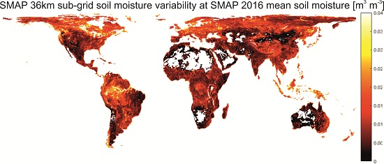
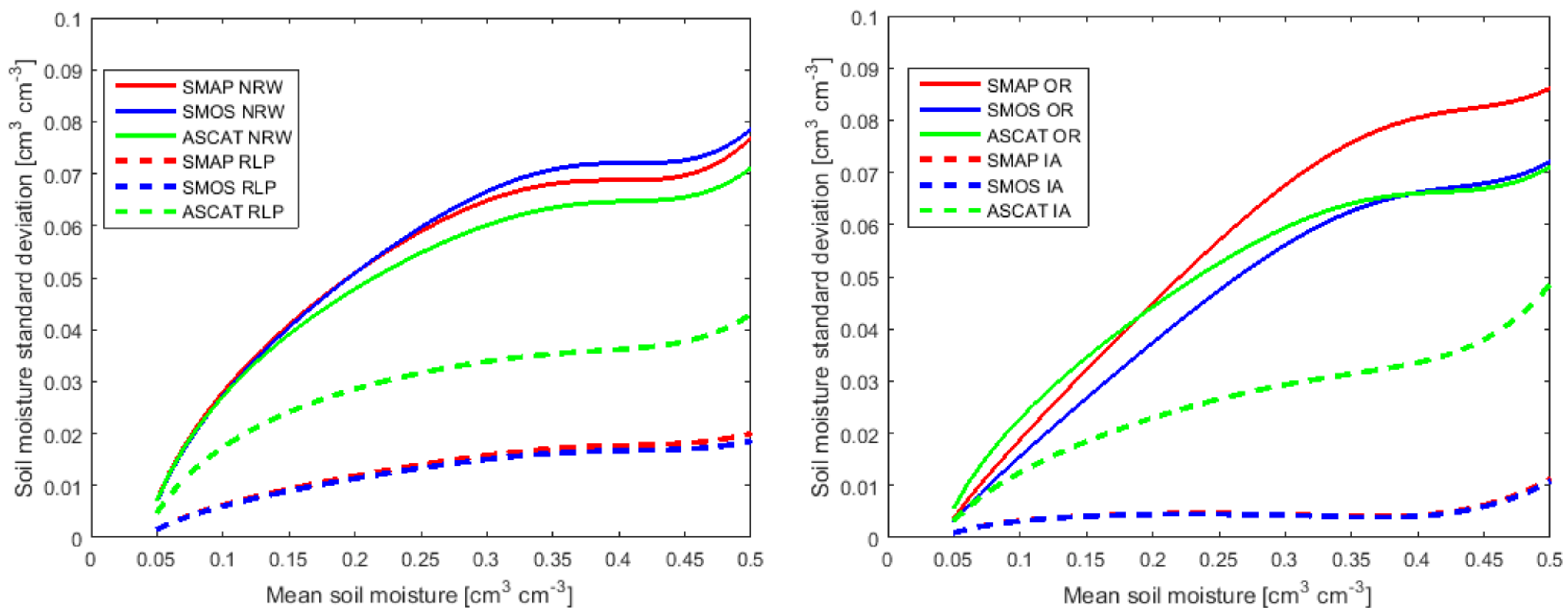
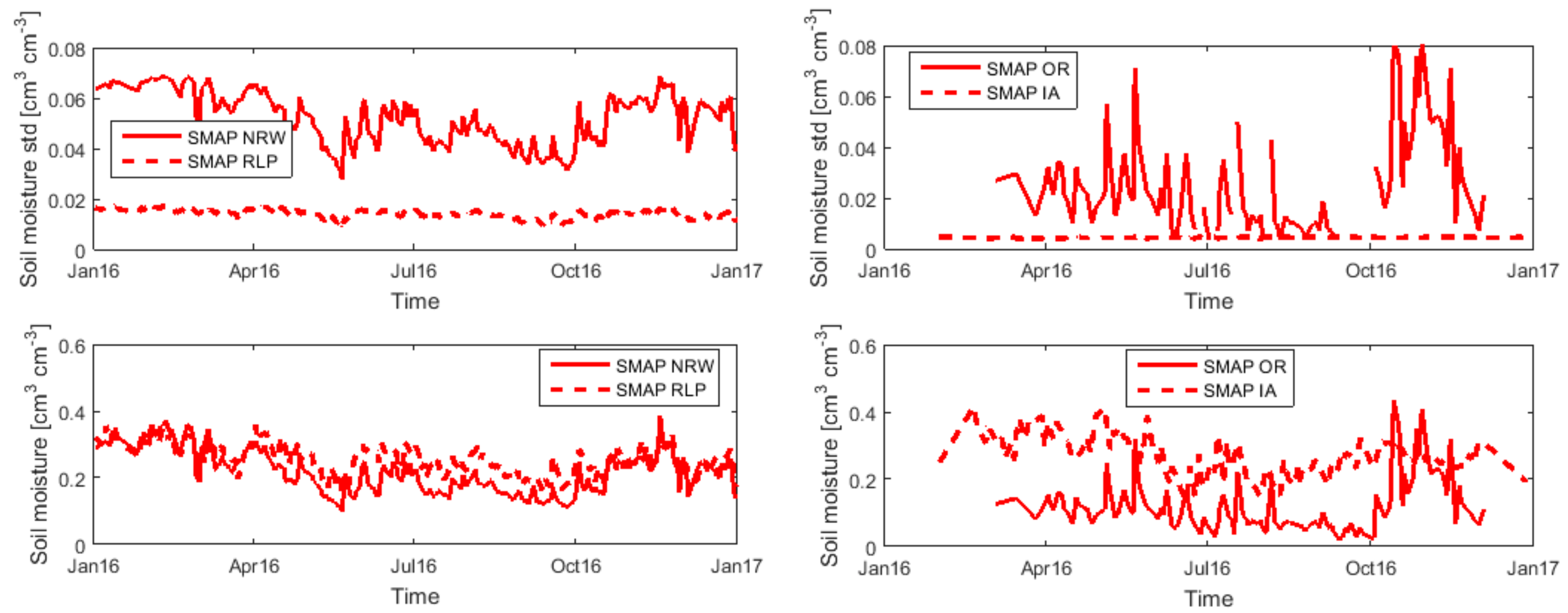
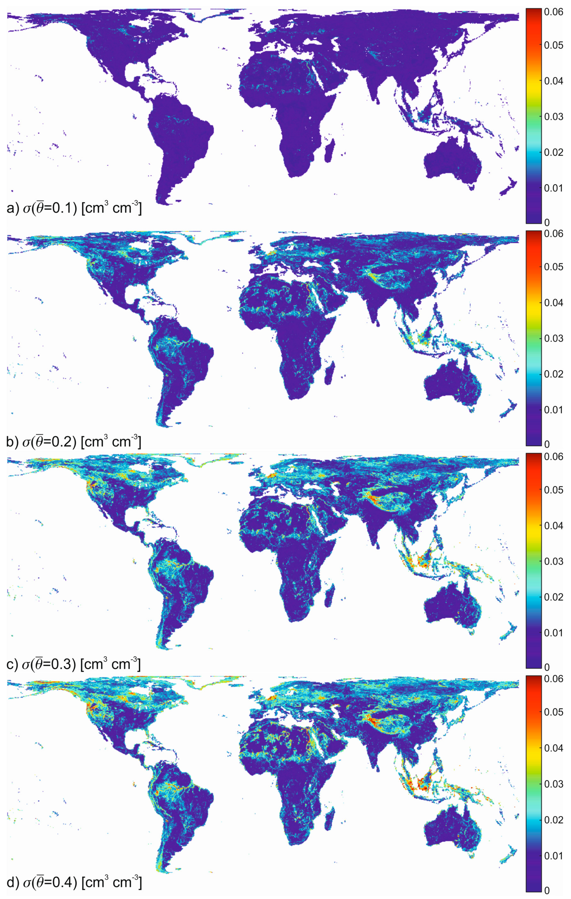
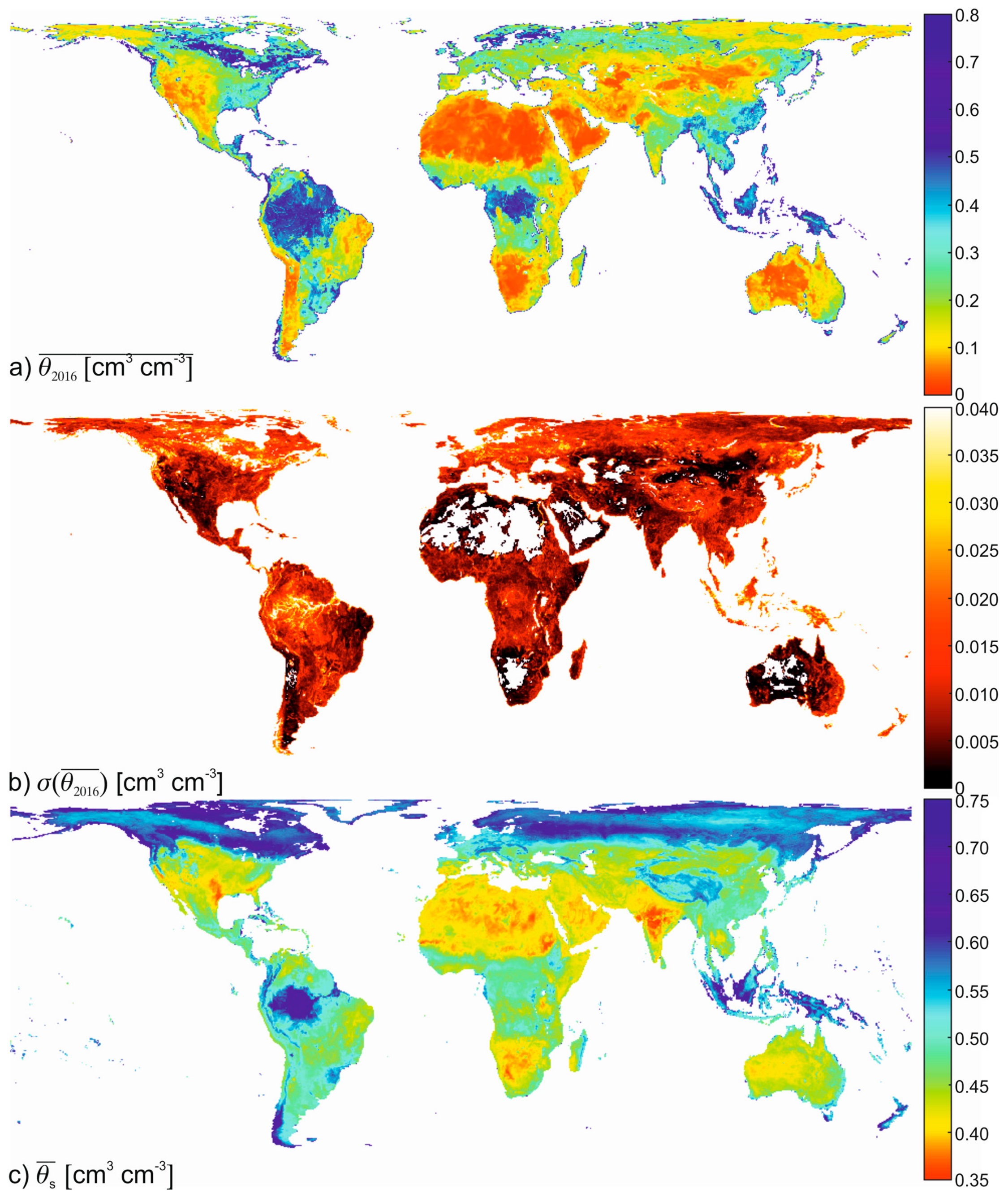
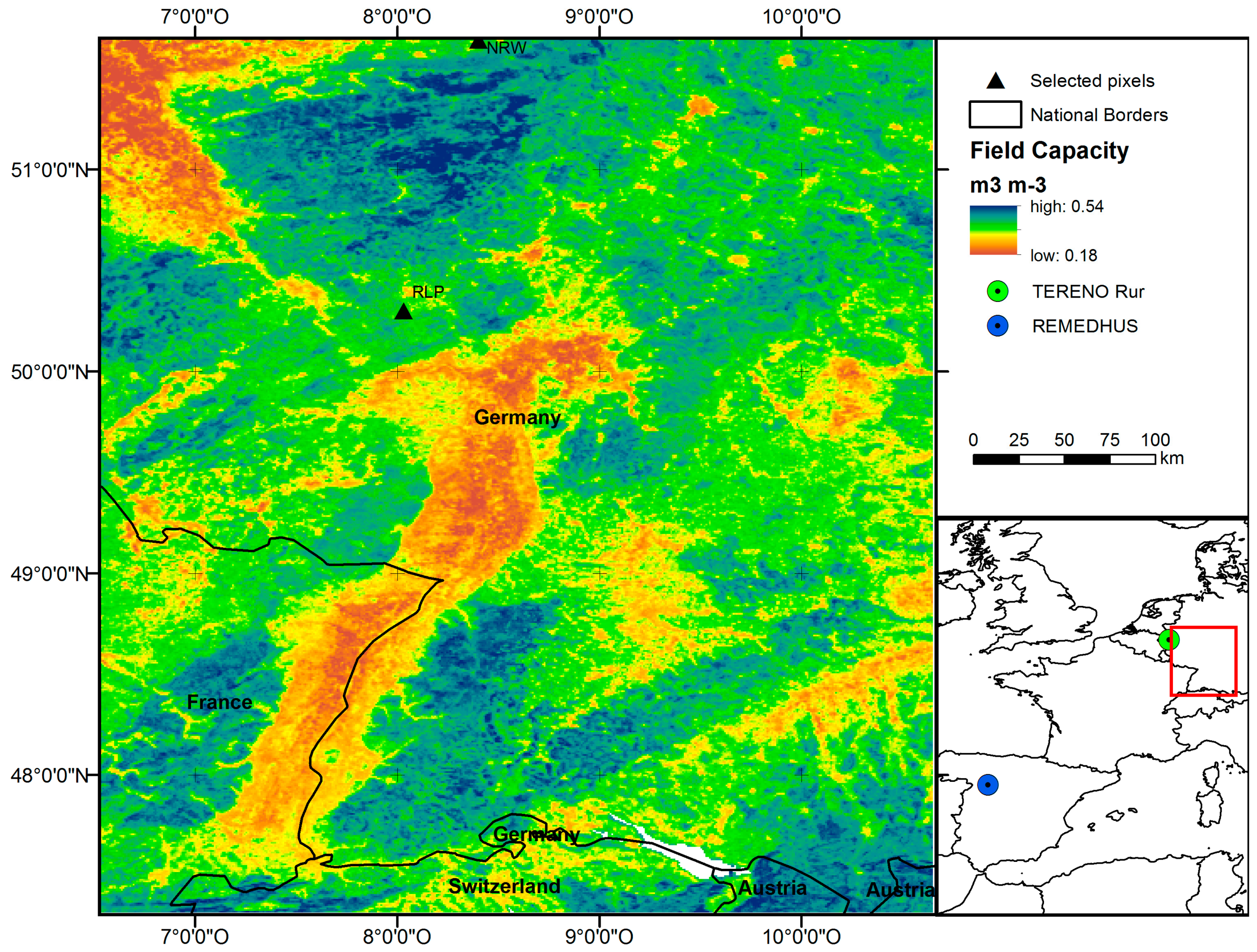
Table 1.
Variables stored in the final data sets.
| Mission | Variable | Unit | Dimensions | Variable Name |
|---|---|---|---|---|
| ASCAT | Grid point index | - | 3,264,391 | gpi |
| Cell number | - | 3,264,391 | cell | |
| Average residual soil water content | cm3 cm−3 | 3,264,391 | mean_thetar | |
| Average saturated soil water content | cm3 cm−3 | 3,264,391 | mean_thetas | |
| Latitude | Decimal degree | 3,264,391 | latitude | |
| Longitude | Decimal degree | 3,264,391 | longitude | |
| Number of valid high resolution pixels | - | 3,264,391 | size_valid | |
| Sub-grid soil moisture standard deviation | cm3 cm−3 | 3,264,391 × 60 | std_theta | |
| Mean soil moisture | cm3 cm−3 | 60 | mean_sm | |
| SMAP | Average residual soil water content | cm3 cm−3 | 406 × 964 | mean_thetar |
| Average saturated soil water content | cm3 cm−3 | 406 × 964 | mean_thetas | |
| Latitude | Decimal degree | 406 | latitude | |
| Longitude | Decimal degree | 964 | longitude | |
| Number of valid high resolution pixels | - | 406 × 964 | size_valid | |
| Sub-grid soil moisture standard deviation | cm3 cm−3 | 406 × 964 × 60 | std_theta | |
| Mean soil moisture | cm3 cm−3 | 60 | mean_sm | |
| SMOS | Average residual soil water content | cm3 cm−3 | 584 × 1388 | mean_thetar |
| Average saturated soil water content | cm3 cm−3 | 584 × 1388 | mean_thetas | |
| Latitude | Decimal degree | 584 | latitude | |
| Longitude | Decimal degree | 1388 | longitude | |
| Number of valid high resolution pixels | - | 584 × 1388 | size_valid | |
| Sub-grid soil moisture standard deviation | cm3 cm−3 | 584 × 1388 × 60 | std_theta | |
| Mean soil moisture | cm3 cm−3 | 60 | mean_sm |
Table 2.
Temporal validation metrics of SMAP downscaling results in the TERENO and REMEDHUS networks. Orig is the original SMAP coarse product, D is the downscaled result, and D/I is the interpolated and downscaled result.
Table 2.
Temporal validation metrics of SMAP downscaling results in the TERENO and REMEDHUS networks. Orig is the original SMAP coarse product, D is the downscaled result, and D/I is the interpolated and downscaled result.
| Site | RMSD | Bias | ubRMSD | R | ||||||||
|---|---|---|---|---|---|---|---|---|---|---|---|---|
| Orig | D | D/I | Orig | D | D/I | Orig | D | D/I | Orig | D | D/I | |
| TERENO Sites | ||||||||||||
| Gevenich | 0.051 | 0.086 | 0.071 | 0.013 | 0.070 | 0.051 | 0.050 | 0.048 | 0.048 | 0.820 | 0.826 | 0.829 |
| Merzen-hausen | 0.053 | 0.041 | 0.061 | 0.030 | −0.005 | −0.049 | 0.043 | 0.041 | 0.037 | 0.803 | 0.799 | 0.817 |
| Ruraue | 0.136 | 0.150 | 0.136 | −0.122 | −0.136 | −0.123 | 0.063 | 0.061 | 0.058 | 0.745 | 0.744 | 0.765 |
| Schone-seiffen | 0.068 | 0.068 | 0.094 | 0.018 | 0.018 | −0.072 | 0.065 | 0.065 | 0.061 | 0.701 | 0.701 | 0.755 |
| Mean | 0.077 | 0.086 | 0.091 | −0.015 | −0.013 | −0.048 | 0.055 | 0.054 | 0.051 | 0.767 | 0.768 | 0.792 |
| REMEDHUS Sites | ||||||||||||
| K10 | 0.086 | 0.077 | 0.086 | 0.075 | 0.067 | 0.072 | 0.042 | 0.037 | 0.046 | 0.889 | 0.890 | 0.879 |
| M5 | 0.037 | 0.033 | 0.034 | 0.013 | 0.008 | 0.005 | 0.035 | 0.032 | 0.034 | 0.901 | 0.901 | 0.897 |
| N9 | 0.052 | 0.062 | 0.062 | −0.039 | −0.052 | −0.052 | 0.035 | 0.033 | 0.033 | 0.895 | 0.898 | 0.904 |
| I6 | 0.121 | 0.117 | 0.122 | 0.105 | 0.101 | 0.105 | 0.060 | 0.057 | 0.062 | 0.815 | 0.815 | 0.809 |
| H7 | 0.129 | 0.117 | 0.136 | 0.115 | 0.106 | 0.121 | 0.058 | 0.052 | 0.062 | 0.865 | 0.867 | 0.876 |
| K9 | 0.058 | 0.048 | 0.055 | 0.045 | 0.035 | 0.041 | 0.036 | 0.033 | 0.038 | 0.873 | 0.879 | 0.868 |
| H9 | 0.184 | 0.197 | 0.180 | −0.168 | −0.180 | −0.164 | 0.075 | 0.081 | 0.073 | 0.917 | 0.916 | 0.923 |
| J14 | 0.035 | 0.033 | 0.032 | −0.005 | −0.006 | −0.008 | 0.034 | 0.032 | 0.031 | 0.934 | 0.931 | 0.930 |
| M9 | 0.082 | 0.086 | 0.089 | −0.063 | −0.070 | −0.072 | 0.052 | 0.049 | 0.052 | 0.731 | 0.730 | 0.726 |
| F6 | 0.096 | 0.102 | 0.086 | −0.082 | −0.091 | −0.072 | 0.048 | 0.046 | 0.046 | 0.784 | 0.787 | 0.822 |
| H13 | 0.061 | 0.058 | 0.057 | −0.036 | −0.021 | −0.034 | 0.049 | 0.054 | 0.046 | 0.888 | 0.887 | 0.886 |
| L3 | 0.060 | 0.047 | 0.056 | 0.036 | 0.024 | 0.031 | 0.048 | 0.041 | 0.047 | 0.885 | 0.884 | 0.879 |
| J12 | 0.151 | 0.146 | 0.154 | −0.144 | −0.139 | −0.148 | 0.044 | 0.044 | 0.042 | 0.875 | 0.874 | 0.864 |
| E10 | 0.051 | 0.050 | 0.049 | −0.002 | −0.003 | 0.014 | 0.051 | 0.050 | 0.047 | 0.788 | 0.788 | 0.852 |
| O7 | 0.041 | 0.043 | 0.052 | 0.025 | 0.028 | 0.039 | 0.035 | 0.033 | 0.035 | 0.870 | 0.870 | 0.874 |
| K4 | 0.119 | 0.112 | 0.114 | 0.106 | 0.100 | 0.102 | 0.054 | 0.049 | 0.052 | 0.905 | 0.906 | 0.907 |
| L7 | 0.061 | 0.063 | 0.067 | −0.053 | −0.056 | −0.060 | 0.030 | 0.029 | 0.030 | 0.919 | 0.920 | 0.919 |
| J3 | 0.112 | 0.104 | 0.113 | 0.102 | 0.095 | 0.103 | 0.047 | 0.042 | 0.046 | 0.935 | 0.939 | 0.938 |
| F11 | 0.073 | 0.076 | 0.077 | 0.055 | 0.059 | 0.062 | 0.048 | 0.047 | 0.045 | 0.927 | 0.924 | 0.936 |
| Mean | 0.085 | 0.083 | 0.085 | 0.004 | 0.000 | 0.005 | 0.047 | 0.045 | 0.046 | 0.873 | 0.874 | 0.878 |
© 2018 by the authors. Licensee MDPI, Basel, Switzerland. This article is an open access article distributed under the terms and conditions of the Creative Commons Attribution (CC BY) license (http://creativecommons.org/licenses/by/4.0/).
Share and Cite
MDPI and ACS Style
Montzka, C.; Rötzer, K.; Bogena, H.R.; Sanchez, N.; Vereecken, H. A New Soil Moisture Downscaling Approach for SMAP, SMOS, and ASCAT by Predicting Sub-Grid Variability. Remote Sens. 2018, 10, 427. https://doi.org/10.3390/rs10030427
AMA Style
Montzka C, Rötzer K, Bogena HR, Sanchez N, Vereecken H. A New Soil Moisture Downscaling Approach for SMAP, SMOS, and ASCAT by Predicting Sub-Grid Variability. Remote Sensing. 2018; 10(3):427. https://doi.org/10.3390/rs10030427
Chicago/Turabian StyleMontzka, Carsten, Kathrina Rötzer, Heye R. Bogena, Nilda Sanchez, and Harry Vereecken. 2018. "A New Soil Moisture Downscaling Approach for SMAP, SMOS, and ASCAT by Predicting Sub-Grid Variability" Remote Sensing 10, no. 3: 427. https://doi.org/10.3390/rs10030427
Note that from the first issue of 2016, this journal uses article numbers instead of page numbers. See further details here.