Estimating Gravimetric Water Content of a Winter Wheat Field from L-Band Vegetation Optical Depth

Abstract

A considerable amount of water is stored in vegetation, especially in regions with high precipitation rates. Knowledge of the vegetation water status is essential to monitor changes in ecosystem health and to assess the vegetation influence on the water budget. In this study, we develop and validate an approach to estimate the gravimetric vegetation water content (m_g), defined as the amount of water [kg] per wet biomass [kg], based on the attenuation of microwave radiation through vegetation. m_g is expected to be more closely related to the actual water status of a plant than the area-based vegetation water content (VWC), which expresses the amount of water [kg] per unit area [m²]. We conducted the study at the field scale over an entire growth cycle of a winter wheat field. Tower-based L-band microwave measurements together with in situ measurements of vegetation properties (i.e., vegetation height, and m_g for validation) were performed. The results indicated a strong agreement between the in situ measured and retrieved m_g (R² of 0.89), with mean and standard deviation (STD) values of 0.55 and 0.26 for the in situ measured m_g and 0.57 and 0.19 for the retrieved m_g, respectively. Phenological changes in crop water content were captured, with the highest values of m_g obtained during the growth phase of the vegetation (i.e., when the water content of the plants and the biomass were increasing) and the lowest values when the vegetation turned fully senescent (i.e., when the water content of the plant was the lowest). Comparing in situ measured m_g and VWC, we found their highest agreement with an R² of 0.95 after flowering (i.e., when the vegetation started to lose water) and their main differences with an R² of 0.21 during the vegetative growth of the wheat vegetation (i.e., where the m_g was constant and VWC increased due to structural changes in vegetation). In addition, we performed a sensitivity analysis on the vegetation volume fraction (δ), an input parameter to the proposed approach which represents the volume percentage of solid plant material in air. This δ-parameter is shown to have a distinct impact on the thermal emission at L-band, but keeping δ constant during the growth cycle of the winter wheat appeared to be valid for these m_g retrievals.

1. Introduction

In the present context of climate change, it is of key importance to closely monitor the vegetation conditions of agricultural fields to secure yield and prevent damage from widespread flood and drought episodes. In this regard, our research aims to develop and validate at the field scale a new approach to retrieve the gravimetric vegetation water content (m_g) from the vegetation attenuation of L-band microwave radiation (τ parameter). Tower-based L-band (1.4 GHz) microwave measurements above a winter wheat field were acquired over an entire growing cycle together with in situ measurements of vegetation properties [1]. The proposed attenuation-based approach to retrieve m_g is built on the τ model of Schmugge and Jackson [2] and on the Debye-Cole dual dispersion dielectric model of Ulaby and El-Rayes [3]. The motivation of our study is to get a direct estimate of the plant water status (i.e., m_g) which, unlike the area-based vegetation water content (VWC), is independent of biomass variations. The VWC can be defined as the amount of water [kg] per unit area [m²] and the gravimetric vegetation water content (m_g) as the amount of water [kg] per wet biomass [kg] [4,5]. The retrieval of VWC was frequently investigated in past studies using optical sensor measurements; global estimates have been validated by using (limited) available in situ measurements (e.g., [6,7]) or by first upscaling ground observations to regional scales via air-borne observations that were later related to space-borne measurements (e.g., [8]). Additionally, several studies were performed at the field scale to retrieve VWC using L-band (e.g., [9] for alfalfa) or a combination of L- and C-band passive microwave measurements (e.g., [10] for soy bean and winter wheat). At L-band, the VWC was shown to be linearly related to the vegetation optical depth (VOD) parameter (τ) [11] using a vegetation structural parameter (i.e., the so-called b-parameter with τ = b ⋅ VWC) [11]. This b-parameter was estimated at the local scale in field studies for multiple vegetation types (e.g., [11,12,13,14]) and has been defined globally for different land cover types based on the International Geosphere-Biosphere Program (IGBP) classification system [15]. However, while the use of b for the retrieval of the VWC is a common and established method considered in ESA’s Soil Moisture and Ocean Salinity (SMOS) [16] and NASA’s Soil Moisture Active Passive (SMAP) [17] retrieval algorithms [12,15], it is not fully physically-based and it is generally defined using empirical methods. In addition, most VWC retrieval approaches were developed at the field scale and require in situ datasets as an input (e.g., vegetation density) [12], which are usually not available on a global scale. Finally, the limited availability of ground measurements makes the validation of globally estimated VWC products very challenging.

The gravimetric vegetation water content (m_g) is expected to be more closely related to the actual water status than VWC and, therefore, better suited for eco-hydrological studies [18]. However, studies addressing the estimation of m_g based on passive microwave measurements are scarce. At the field scale, the m_g was shown to be highly dependent on the absorption and the scattering of microwave emissions at L-, C-, and X-bands for leaves of a soybean canopy [13]. In addition, a strong relationship to the complex vegetation dielectric constant (ε_veg) for different plant parts (i.e., stalks and leaves of wheat and corn plants [14] or wheat heads [19]) was reported. A few studies proposed approaches for the global estimation of m_g from τ estimates [5,18]. However, the retrieval of m_g still needs further investigation and improvement, especially at the global scale, since in situ reference datasets for validation are also missing at this scale [18,20]. In particular, a proper characterization of the canopy volume is a pre-requisite information to estimate m_g. Such information is generally unknown and often fixed as a constant or neglected in actual retrieval algorithms (e.g., the τ-ω model [21]). The vegetation volume fraction (δ) can be defined as the volume percentage of solid plant material of a canopy in air [22]. The δ-parameter has a high impact on the emission-band radiation originating from the vegetation and is therefore directly related to water absorption within the canopy [13]. Thus, an improved estimate of δ may lead to more accurate estimates of the attenuation of microwave emissions by the vegetation layer [2,13], and therefore more accurate estimates of m_g. Only a few field studies have investigated δ so far. They state that δ typically ranges between 0 and 0.01 for most vegetation layers [2] and that it can in general be assumed to be smaller than 0.01, like that shown by Wigneron et al. [13] for a soybean canopy. The objectives of our study are to investigate the information on water content and above-ground biomass contained in the vegetation optical depth parameter and to develop an algorithm to extract m_g from τ under controlled field experiment conditions.

The decision to use L-band data was made as the L-band is a promising frequency to monitor crop vegetation, as it penetrates into the canopy (i.e., measurements of the whole above-ground plant layer are possible), is less affected by scattering within the vegetation than higher frequencies, and is located within a protected band leading to low radio frequency interference (RFI) [23]. However, the L-band is more sensitive to soil moisture than higher frequencies, especially if the vegetation density is low to moderate. C- and X-band radiometer measurements (e.g., as provided by AMSR-E and WindSat) are less sensitive to the soil moisture content and could be better suited to characterize the (upper) vegetation layer [24,25]. Nonetheless, we performed our measurements in the L-band for the reasons given above, and designed our experiment specifically to block the soil surface emission and thus avoid the soil moisture influence on the radiometer measurements. Furthermore, vegetation indices retrieved from passive L-band measurements differ from indices deducted from optical or active microwave observations. Optical sensors do not penetrate into the canopy and only sense the very top of the vegetation layer (leaf component) [4]. Active microwave sensors, in turn, are more strongly affected by scattering within the vegetation than their passive counterparts [26,27]. Passive microwave observations at L-band allow to estimate the vegetation permittivity (dielectric constant), which can be directly related to properties, like water content, density, and structure [28,29]. In this context, the vegetation water status is a key variable for global and regional climate models to improve water budget estimations [30,31].

The following research questions were investigated during our study: (a) Can we retrieve the gravimetric moisture (m_g) of vegetation using the vegetation optical depth (τ) parameter, i.e., the degree to which vegetation attenuates microwave radiation in the L-band?; (b) Is m_g influenced by changes of the vegetation canopy (e.g., structure, biomass) over the growing season of a winter wheat field?; (c) Is the retrieval of m_g influenced by the applied vegetation dielectric mixing model (i.e., assuming different vegetation shapes in the dielectric mixing model)?; and (d) Is the assumption of a constant δ valid for the retrieval of m_g at the field scale?

Section 2 presents the experimental setup and the methodology of the microwave attenuation-based approach to estimate m_g. Section 3 shows the results of the retrieved m_g and its correlation to in situ measured m_g. Additionally, a sensitivity analysis of m_g for varying δ is presented, as well as a comparison between the in situ measured m_g and the in situ measured VWC values. In Section 4, we discuss the results of the m_g-retrieval, our findings concerning the δ-parameter, and the potential of our attenuation-based approach to provide estimates of m_g. Section 5 provides a summary and our conclusions.

2. Materials and Methods

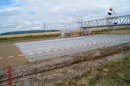
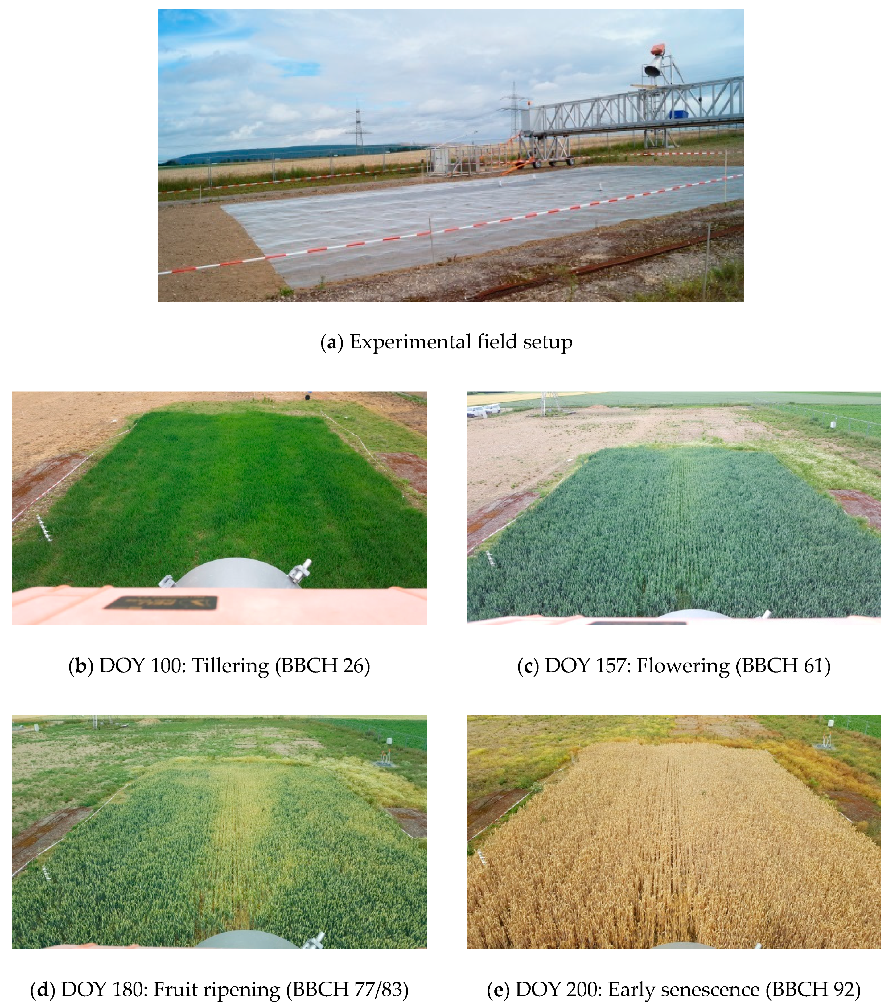
2.1. Experiment Description, Vegetation Conditions, and Datasets

Tower-based passive microwave measurements over a winter wheat (Triticum aestivum L.) field were carried out using the ELBARA-II radiometer during summer 2017 [1]. The measurements were performed at the Selhausen remote sensing field laboratory (Germany) [21]. The ELBARA II device operates in the L-band with a center frequency of 1.4 GHz. The measurements were performed at horizontal (p = H) and vertical (p = V) polarization (p) using a 3 s integration time to provide an accuracy of about 1 K and the −3 dB full beam width was 23° in the far field. The radiometer was mounted on an aluminum bridge at about 4 m height.

The experiment was conducted during a period of about four months from tillering of the winter wheat on April 10th (DOY 100) to the late senescence stage on August 14th (DOY 226). The microwave measurements were performed twice a week over a gridded plot (i.e., soil covered by a perfect reflector (metal grid) to block the soil surface emission, but allowing vegetation to grow through the mesh grid) for different incidence angles (i.e., 40–60° in increments of 5°) during the morning (i.e., from 8 to 12 a.m.). The collected brightness temperature (T_B) data showed that the T_BV measurements had a higher temporal variability with generally higher values over the entire growing period, and also a larger increase and dynamic range during crop development, compared to T_BH (e.g., a STD of 18.4 K for T_BH and 53 K for T_BV using a 40° incidence angle). This can be explained by the stronger vertical orientation of the wheat canopy leading to a higher emission contribution in the V polarization [1]. In addition, weekly in situ measurements of vegetation properties were performed for: leaf area index (LAI), total above ground biomass (TOB), vegetation water content (VWC), growing stages (BBCH), and vegetation height (d). The field experimental setup and the changes in the vegetation layer during the growing season are depicted in Figure 1 for selected phenological stages. The vegetation layer changed significantly during the phenological cycle of the winter wheat plants with a leaf-dominated vegetation structure between DOY 100 and 120, followed by a period of stalk-dominated vegetation structure (DOY 120–180) where the highest VWC was reached during flowering, and a period where the vegetation turned into senescence (DOY ≥ 200) and the heads as well as the stems of the wheat began to bend towards the soil surface. For a more detailed description of the field setup and the collected measurement datasets (i.e., in situ and radiometer) see Meyer et al. [1].

In the current study, we used the polarization (p) dependent vegetation optical depth (τ) parameter, which was retrieved from the 40° incidence angle brightness temperature measurements using the τ–ω model [32]. Optimal values for τ (H and V polarizations) were simultaneously estimated for one measurement angle using T_B data at both polarizations. Additionally, information on canopy temperature (measured at 15 cm above ground) was used. The T_B data consisted of mean values of the five measurements performed per day (n = 33 days, from which only 20 measurement days correspond to the in situ measured vegetation properties) at the 40° incidence angle and for each polarization. The estimated τ_V as well as in situ measurements of vegetation height (d) were used as an input in our m_g retrieval approach. Finally, to be able to compare our retrievals of m_g with a reference dataset, the in situ VWC was converted to m_g by calculating first the dry matter fraction (m_d) as defined by Mätzler [33] (i.e., m_d = $\frac{dry mass}{fresh mass}$) and subtracting it afterwards from 1 (i.e., $m_g=1-m_d$). This calculated m_g will be called in situ measured m_g in our study.

2.2. Methodology for Estimating the Gravimetric Water Content of Vegetation

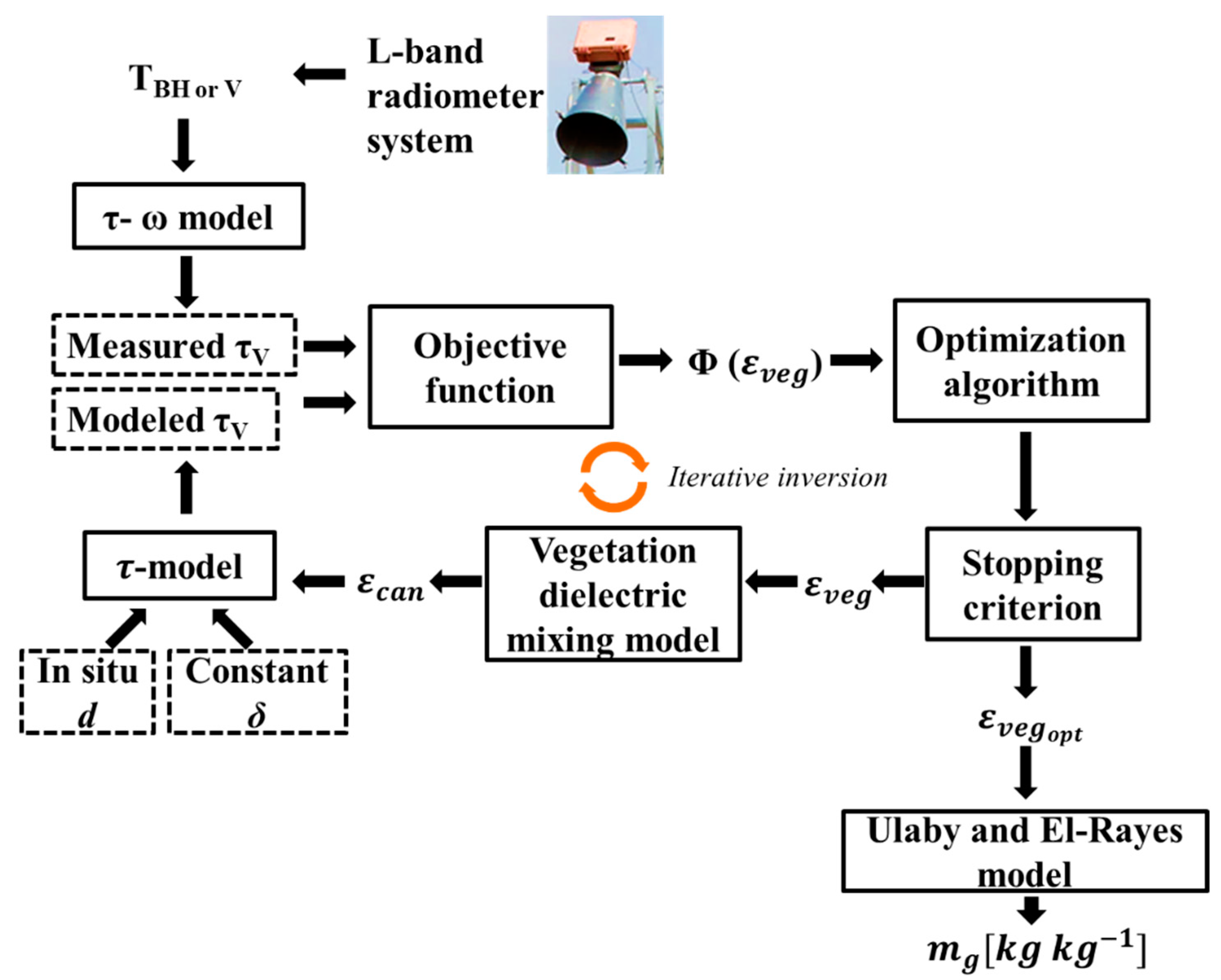
2.2.1. Retrieval Algorithm

Figure 2 shows, conceptually, the retrieval scheme of m_g. For the estimation of m_g, the in situ measured vegetation height (d), a constant value of the vegetation volume fraction (δ), and the canopy dielectric constant (ε_can) (i.e., which was derived from the modelled complex vegetation dielectric constant (ε_veg)) were used as input for the τ model. The output modelled τ values were then compared to the radiometer-derived τ values (i.e., which were estimated from L-band brightness T_B measurements using the τ–ω model (see Section 2.1) by minimizing the objective function (φ), which is defined as the cumulative squared error between the modelled and measured τ. Finally, the optimal (opt) ε_veg is obtained from the best fit between τ-model and the radiometer-derived τ, and is converted to m_g using the model of Ulaby and El-Rayes [3]. The different vegetation dielectric mixing models used to estimate ε_can will be explained in Section 2.2.2. In addition, further explanations regarding the conversion of the ε_veg to the corresponding m_g and vice versa will follow in Section 2.2.3.

Concerning the radiometer-derived τ parameter, τ_p at vertical (p = V) polarization was used for the m_g retrieval as τ at horizontal polarization (p = H) did not lead to a proper estimation of m_g (i.e., a significantly deviating temporal evolution and underestimation of m_g in comparison to the in situ measured m_g (results not shown)). The fact that τ_V performed better for the m_g retrieval can be explained by the strong vertical structure of the wheat canopy which is better sensed with V- than with H-polarization. Therefore, all results presented in this work are only based on one polarization (i.e., V-polarization) and one incidence angle (i.e., 40°). Using τ at nadir (τ_NAD) (i.e., corrected for anisotropy) retrieved from multiple incidence angles was not an option, as the resulting estimated m_g showed a similar behavior as the m_g for the τ_H-case in comparison to the in situ measured m_g. To minimize φ during the m_g-retrieval, the multi-level coordinate search (MCS) algorithm [34] was used. Additionally, we used the Local–Nelder–Mead simplex algorithm [35] to further improve the optimization.

Concerning δ, it is not directly measurable with the radiometer and was not measured in the field. It could be estimated from radar measurements using the Radar Vegetation Index (RVI) (e.g., as proposed in [18]) but, unfortunately, radar measurements were not performed during this experiment. Hence, we performed a sensitivity analysis to assess whether it was reasonable to set δ to a constant value along the entire growing period. Note a daily retrieval of δ was not possible (i.e., a global minimum could not be found and several δ-values led to the smallest φ (local minima)). A range of literature values for constant δ (between 0 and 0.01 [18,20]) were tested in the m_g retrieval approach and the δ which led to the smallest φ was chosen based on a model selection. The search step for finding the optimum δ for the entire growing period was set to 10⁻⁶, to ensure that the global minimum could be found. Finally, a sensitivity analysis was performed where the influence of the constant δ-parameter assumption on the estimated m_g using the attenuation-based approach was investigated (as presented in Section 3.2).

The proposed attenuation-based m_g-retrieval concept was first applied in a previous study to global SMAP radiometer data for τ estimation and radar for δ estimation [5]. It has been adapted here for application at the field scale. Note that it was not possible to retrieve both parameters simultaneously, since V-polarization data at one incidence angle (i.e., 40°) does not contain enough information to retrieve two variables simultaneously (i.e., m_g and δ) (see Section 4).

2.2.2. Modelling the Vegetation Optical Depth Including a Two-Phase Dielectric Mixing Model

Our approach is based on the attenuation model proposed by Schmugge and Jackson [2]. They found that for a wavelength (λ) [m] at frequencies between 0.2 and 20 GHz the nadir vegetation optical depth VOD (τ) can be related to the imaginary part of the complex dielectric constant of the canopy (ε_can) by:

$$\tau =4\pi \left(\frac{d}{\lambda }\right). Im\left[\sqrt{{\epsilon }_{can}}\right],$$

(1)

where the square root of ε_can is applied, since it is directly related to the refractive index of the canopy, and the imaginary part (Im) (also called loss factor) refers to the loss of the electromagnetic energy when the waves propagate through a vegetation layer with thickness d [m]. Thus, τ describes the attenuation of the surface emission when it passes through the vegetation canopy. For the description of ε_can, different two-phase dielectric mixing models can be used, as proposed by de Loor [36] who extended the work of Polder and van Santen [22] on the dielectrics of mixtures of solids. Thus, the vegetation layer can be described as a two-phase mixture with air as the host material with a dielectric constant (ε_air) equal to one and the vegetation as inclusions with a specific shape (i.e., spheres (s), needles (n), discs (di)), orientation (i.e., random (r) or vertical (v)), complex vegetation dielectric constant (ε_veg), and volume fraction (δ). For the winter wheat field, the vertical needles (vn) dielectric mixing model is expected to perform best to retrieve m_g, as the winter wheat canopy is mainly vertically oriented (distinct stalk component) and therefore anisotropic attenuation effects should be significant. The randomly-oriented discs (rdi) dielectric mixing model will also be tested as the leaves have a disc like shape without a dominant orientation (i.e., random). The equations used to calculate ε_can for vegetation inclusions with vertical needles (vn) and randomly-oriented discs (rdi) can be found in [19]. For the vertically oriented needles (vn) inclusions:

$${\epsilon }_{can} ={\epsilon }_{host}+\frac{\delta }{3}\left({\epsilon }_{ve{g}_{}}-{\epsilon }_{host}\right){\displaystyle \sum }_{u=a,b,or c}\left(\frac{1}{1+A_u\left(\frac{{\epsilon }_{ve{g}_{}}}{{\epsilon }_{host}}-1\right)}\right),$$

(2)

where ε_host is the dielectric constant of the host material (which is equal to ε_air in the case of a canopy layer in nature) and the so-called shape factor (A_u) (also called depolarization factor) which describes the influence of the inclusion shape on the dielectric constant along its semi-axis (u = a, b, or c). The semi-axes a and b are symmetric in the vn mixing model (i.e., a = b) and c >> a. The A parameter is than A_a = A_b = 0.5 and A_c was set equal to zero in our case because we did not perform measurements of the stalk diameter to calculate the ellipsoid eccentricity. The sum of the three shape factors is always equal to 1 [19]. When assuming that the vegetation inclusions have the shape of randomly oriented discs (rdi) the semi-axes are a = b and c << a and the following equation should be used:

$${\epsilon }_{can} ={\epsilon }_{host}+\frac{\delta }{3}\left({\epsilon }_{veg}-{\epsilon }_{host}\right)\left(2+\frac{{\epsilon }_{host}}{{\epsilon }_{veg}}\right).$$

(3)

The A-parameter can be assumed to be equal to A_a = A_b = 0 and A_c = 1, in this case. In general, it has to be stated that for vegetation layers with an anisotropic structure, vegetation dielectric mixing models which account for the orientation (i.e., random or vertical) and the shape of the inclusions (i.e., needles or discs) seem to perform better at the field scale (e.g., [13]) than mixing models which do not account for the orientation and shape of the vegetation inclusions (i.e., assuming the shape of spheres) [5]. Hence, the choice of the dielectric mixing model should be adapted to the actual phenological stage and the vegetation species. In addition, it is also important to mention that on large scales (kilometer resolution of radiometers) the vertical and horizontal structure in natural vegetation are usually mixed and do not appear monotonically oriented over large areas. In these cases, dielectric mixing models which describe the vegetation as isotropic structures would describe the vegetation layer in a more appropriate way (i.e., the spheres (s) or random needles (rn) mixing models [19]), as was shown by Fink et al. [5] using SMAP data. However, for our field scale study on a single winter wheat field, s and rn dielectric mixing models did not succeed in representing the anisotropic structure of the wheat stalks and will, therefore, not be considered here.

2.2.3. Conversion of Vegetation Dielectric Constant into Gravimetric Vegetation Water Content

Ulaby and El-Rayes [3] developed the semi-physical Debye–Cole dual-dispersion dielectric mixing model. It is a low-parameterized and well-established model to convert the gravimetric vegetation water content (m_g) [kg kg⁻¹] into the corresponding complex vegetation dielectric constant (ε_veg) and vice versa (e.g., applied by [13,37]). It assumes that ε_veg is a mixture of three components [3]: a non-dispersive residual component r [–], a free-water component fw [–], and a bulk vegetation-bound water component b [–]. These three components in turn depend on m_g. Therefore, ε_veg can be defined as [3]:

$${\epsilon }_{veg}={\epsilon }_r + v_{fw}{\epsilon }_{fw}+ v_b{\epsilon }_b,$$

(4)

where ${\epsilon }_r$ is the nondispersive residual component of the complex dielectric constant, with the following equation:

$${\epsilon }_r=1.7-0.74m_g+6.16m_g{}^2.$$

(5)

The ${\epsilon }_{fw}$ and ${\epsilon }_b$ of Equation (4) are the free-water and the bulk vegetation bound water components of the complex dielectric constant, respectively. They are defined as follows:

$${\epsilon }_{fw}=4.9+\frac{75.0}{1+jf/18}-j \frac{18\sigma }{f},$$

(6)

$${\epsilon }_b=2.9+\frac{55.0}{1+{\left(jf/0.18\right)}^{0.5}},$$

(7)

where $f$ is the measurement frequency [GHz] and $\sigma$ is the ionic conductivity of the aqueous solution [S m⁻¹] ($\sigma$ is assumed to be equal to 1.27 as in Ulaby and El-Rayes [3]). $j$ denotes the imaginary number. $v_{fw}$ and $v_b$ of Equation (4) are the associated volume fractions of the free-water and bound vegetation bound-water mixture, respectively. They are described as:

$$v_{fw}=m_g\left(0.55m_g-0.076\right) ,$$

(8)

$$v_b=\frac{4.64m_g{}^2}{\left(1+7.36m_g{}^2\right)}.$$

(9)

Furthermore, parameters in Equation (4) depend on frequency, temperature, and salinity. As suggested in [3], plant temperature and salinity are fixed to 22 °C and 10‰, respectively. This allows keeping the conversion static and avoids the need of accounting for any additional bias in the subsequent analysis. By using Equatoin (4) any value of m_g (between 0 and 1) can be associated to a certain value of ε_veg and vice versa.

3. Results

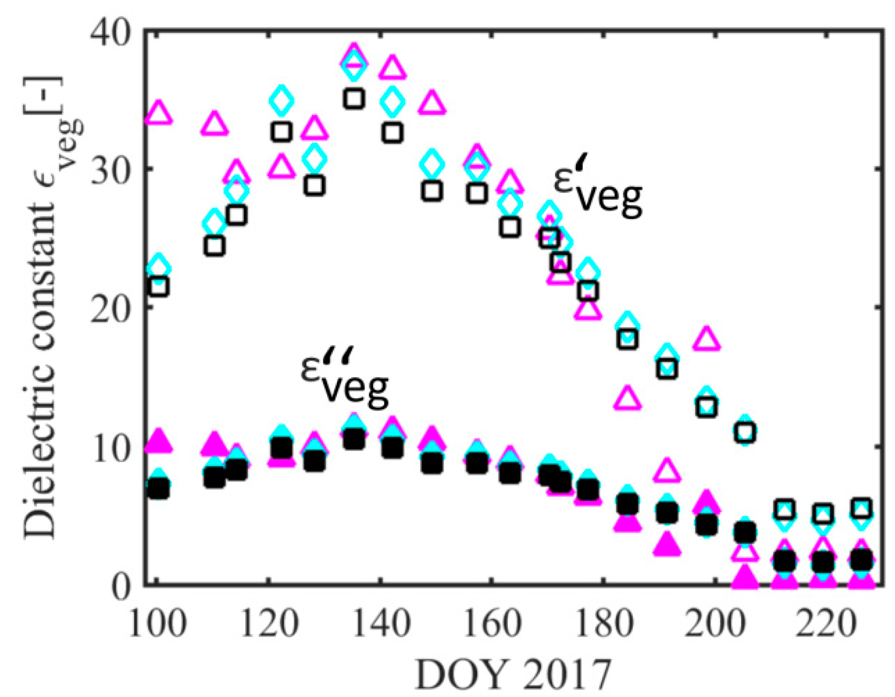
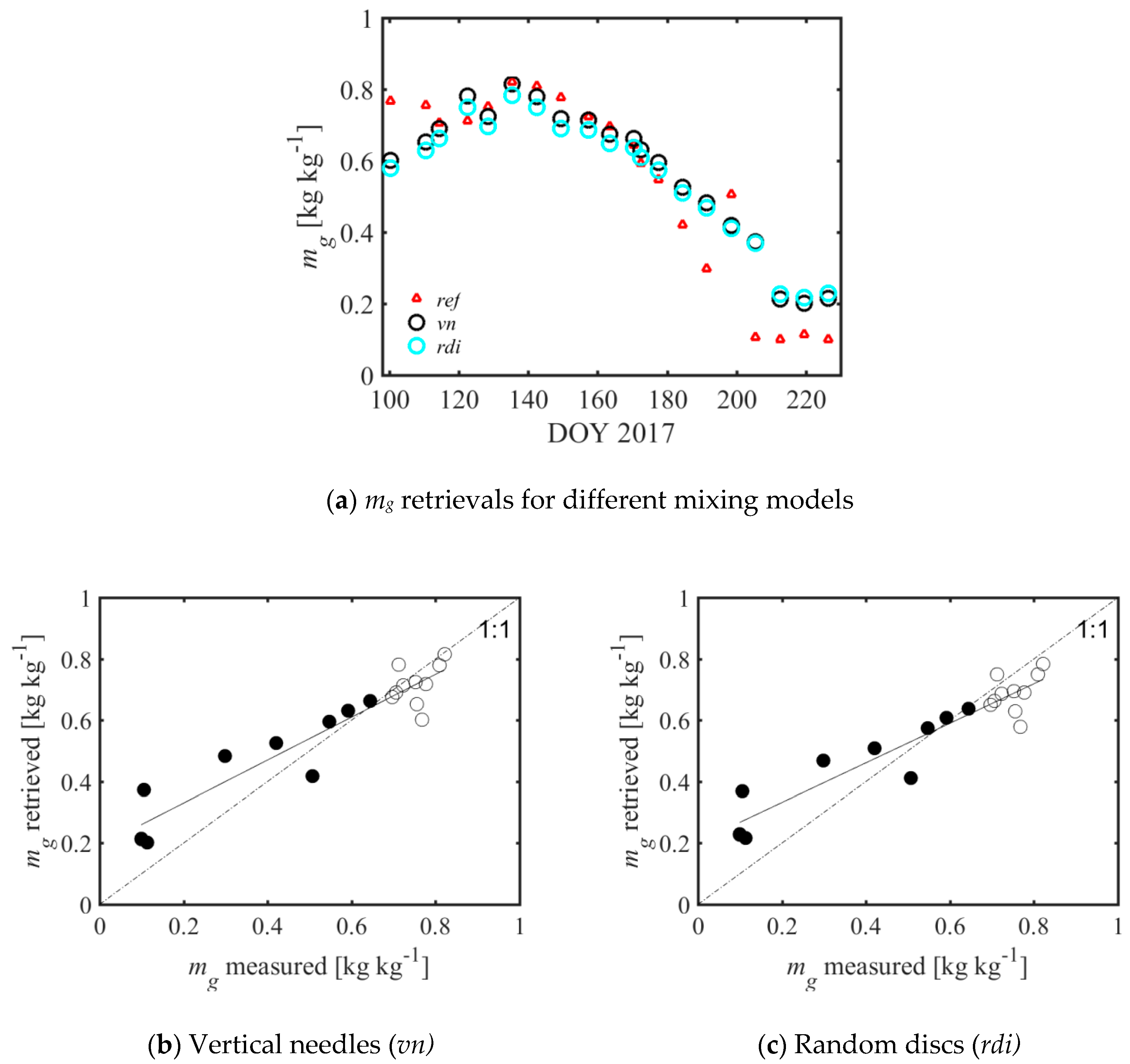
3.1. Gravimetric Vegetation Water Content Retrieval

The complex dielectric constant of vegetation (ε_veg) will be analyzed (before conversion to m_g, see Figure 2) to illustrate the dielectric variation with changing vegetation water content. Figure 3 depicts the estimated ε_veg values for the vertical needles (vn) (open and filled black squares) and random discs (rdi) (open and filled cyan diamonds) dielectric mixing model (retrieved from V polarization data only) and the ε_veg values derived from in situ measurements as a reference (open and filled magenta triangles). The real and imaginary parts of the ε_veg (i.e., ${\epsilon }_{veg}^{\prime }$ and ${\epsilon }_{veg}^{″}$, respectively) show for both mixing models an increase of the ε_veg between DOY 100 and 140 reaching a peak value around DOY 140 of about 35 (${\epsilon }_{veg}^{\prime }$) and 10 (${\epsilon }_{veg}^{″}$), respectively, and a decrease of ε_veg afterwards to minimum values around 6 (${\epsilon }_{veg}^{\prime }$) and 4 (${\epsilon }_{veg}^{″}$), respectively, at the end of the experiment (senescence phase). In comparison to the in situ measured ε_veg (which were converted from the in situ measured m_g using the Ulaby and El-Rayes model [3]) the modeled ε_veg seems to be underestimated during the beginning of the experiment (i.e., between DOY 100 and 120) and overestimated during the senescence phase (i.e., after DOY 180). The mean and STD values of the modelled and measured ε_veg can be found in

Table 1. Mean and standard deviation (STD) values of modelled ${\epsilon }_{veg}^{\prime }$ (real part) and ${\epsilon }_{veg}^{″}$ (imaginary part) using the vertical needles (vn) and random discs (rdi) dielectric mixing model in comparison to ${\epsilon }_{veg}^{\prime }$ and ${\epsilon }_{veg}^{″}$ derived from in situ measurements.

	vn		rdi		In Situ
	${\mathit{\epsilon }}_{\mathit{v}\mathit{e}\mathit{g}}^{\prime }$	${\mathit{\epsilon }}_{\mathit{v}\mathit{e}\mathit{g}}^{\prime \prime }$	${\mathit{\epsilon }}_{\mathit{v}\mathit{e}\mathit{g}}^{\prime }$	${\mathit{\epsilon }}_{\mathit{v}\mathit{e}\mathit{g}}^{\prime \prime }$	${\mathit{\epsilon }}_{\mathit{v}\mathit{e}\mathit{g}}^{\prime }$	${\mathit{\epsilon }}_{\mathit{v}\mathit{e}\mathit{g}}^{\prime \prime }$
mean	22.5	7.0	22.2	6.8	21.3	6.7
STD	10.3	3.0	12.8	3.9	9.4	2.8

.

The obtained ε_veg values are comparable to vegetation dielectric constant values found for crops in literature. Ulaby and Jedlicka [14] performed measurements of the dielectric properties of wheat and corn leaves and stalks at a frequency of 1.5 GHz and found values between 2.5 and about 35 for ${\epsilon }_{veg}^{\prime }$ and values between 0 and about 10 for ${\epsilon }_{veg}^{″}$.

The complex (i.e., real (${\epsilon }_{veg}^{\prime }$) and imaginary part (${\epsilon }_{veg}^{″}$) of the) vegetation dielectric constant was considered in the dielectric mixing model to calculate ε_can, which was used as an input in Equation (1) (i.e., the τ-model). After minimization, Figure 4a depicts the estimated m_g using different vegetation dielectric mixing models (i.e., vn and rdi) as well as the in situ measured m_g (ref) as a reference. In addition, linear regressions between the in situ measured and retrieved m_g using the vn and the rdi dielectric mixing model are shown in Figure 4b,c, respectively.

Table 2. Slope, intercept, and squared Pearson correlation coefficient (R²) values of the linear regression between measured and modelled m_g using the vn and rdi dielectric mixing models. Furthermore, the bias and RMSE between the measured and retrieved m_g are shown.

		Slope	Intercept	R2	Bias	RMSE
Modelled mg (vn)	Measured mg	0.70	0.19	0.89	0.03	0.10
Modelled mg (rdi)	Measured mg	0.64	0.20	0.89	0.009	0.11

contains the corresponding slope, intercept, and squared Pearson correlation coefficient (R²) values of the linear regression analysis. As can be seen for both the vn and the rdi dielectric mixing models, there is good agreement between measured and modelled m_g, with an R² of 0.89 and root mean square error (RMSE) values of 0.10 and 0.11, respectively, showing a mean and STD of 0.57 and 0.19 (vn) and 0.55 and 0.18 (rdi). The mean and STD of the in situ measured m_g are 0.55 and 0.26, respectively. The smallest bias can be found for the rdi mixing model with a value of 0.009. However, the vn and rdi models still underestimate the in situ m_g between DOY 100 and 120 and overestimate m_g after DOY 180. This is probably due to the fact that we had to assume a constant value of δ over the whole growing period due to an insufficient number of measurements, i.e., too low degree of information, to determine δ, whilst knowing that, in reality, the volume/structure of the vegetation is actually changing along with the phenological development.

This can be also seen in the linear regression plots (Figure 4b,c), where the retrieved m_g during the vegetative growth stages (i.e., open black circles) are located below (underestimation) and the retrieved m_g during the senescence stages (i.e., filled black circles) are located above (overestimation) the ideal correlation (1:1) line. Concerning the slopes and intercepts of the regression lines, the vn dielectric mixing model shows a slightly closer fit to the 1:1 line.

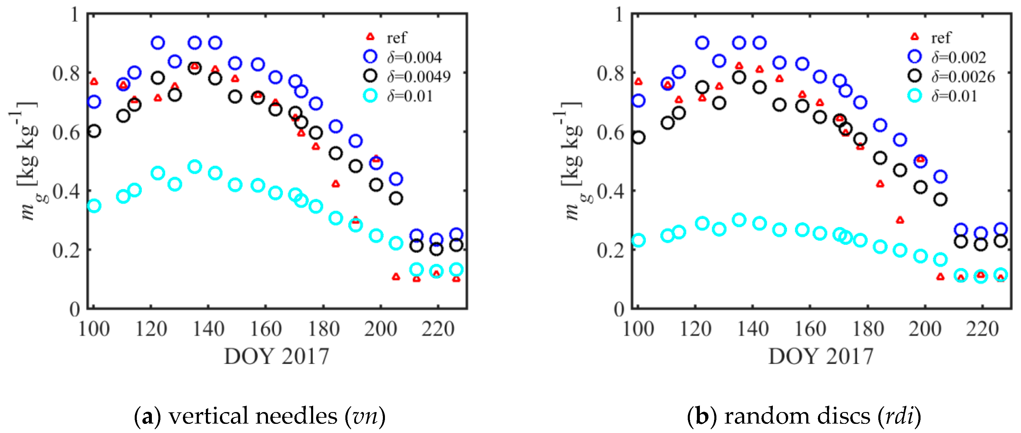
3.2. Sensitivity Analysis on the m_g Retrieval for Varying δ

Numerical experiments were conducted to analyze the impact of assuming a constant δ on m_g-retrievals. Figure 5 depicts the results of the m_g-retrieval along the growing season using the vertical needles (vn) (a) and random discs (rdi) (b) dielectric mixing models with the in situ measured m_g-values (ref) as a reference, for different values of δ. Results show that mean and STD values of m_g steadily decrease for increasing δ (see also

Table 3. Mean and STD values of retrieved m_g [kg kg⁻¹] for selected δ-values using the vertical needles (vn) and random discs (rdi) dielectric mixing models (cf. Figure 5) and the mean and STD of the in situ measured m_g as reference (ref).

	δ-Values	Mean—mg	STD—mg
vn	0.004	0.66	0.22
	0.0049	0.57	0.19
	0.01	0.34	0.11
rdi	0.002	0.67	0.22
	0.0026	0.55	0.18
	0.01	0.22	0.06
ref	-	0.55	0.26

). When using the vn or rdi mixing model, a high δ (i.e., 0.01) leads to an underestimation of m_g and if δ is low (i.e., 0.004 (vn) or 0.002 (rdi)) m_g is overestimated. A δ of 0.0049 (vn) or 0.0026 (rdi) leads to the minimum in the objective function φ between the measured and modelled τ_V (but this minimum is not unique as mentioned before in Section 2.2.1) and to the closest fit between the retrieved and in situ measured m_g. However, in general, there is no large difference in the temporal behavior of the retrieved m_g when using the vn and rdi dielectric mixing models while varying δ. Concerning the m_g-value range, it can be seen that m_g ranges between ~0.2–0.45 for δ equal to 0.01 and ~0.25–0.95 for δ equal to 0.004 for the vn model and almost in the same range for the rdi model with m_g values between ~0.15 and 0.3 for δ equal to 0.01 and ~0.25 and 0.95 for δ equal to 0.002.

Interestingly, the vn model seems to be in general more sensitive to changes of δ than the rdi mixing model. This can be seen in the fact that δ for the vn model was only varied between 0.004 and 0.01 and for the rdi dielectric mixing model δ was varied between 0.002 and 0.01 showing almost the same changes in estimated m_g. Yet, it is important to note that small changes of δ result in relatively large changes in retrieved m_g.

In general, the highest sensitivity of the m_g-retrieval using either the vn or rdi dielectric mixing models to changes of δ can be found between DOY 100 and 180 (i.e., when the m_g-values are relatively high with values between 0.8 and 0.5) and the lowest sensitivity appears during the senescence phase (i.e., when the m_g-values are very low (≤0.25)). This means that the effect of δ on the L-band microwave thermal emission is higher when also the water content of the plants is high (e.g., varying δ between 0.002 and 0.01 decreases the mean value of m_g by about 0.56 for the rdi mixing model at DOY ≤ 160). For lower water contents (i.e., low m_g-values at DOY > 200) the effect of δ on the thermal emission can be assumed to be rather small (e.g., varying δ between 0.002 and 0.01 decreases the mean value of m_g by ~ 0.2 for the rdi model).

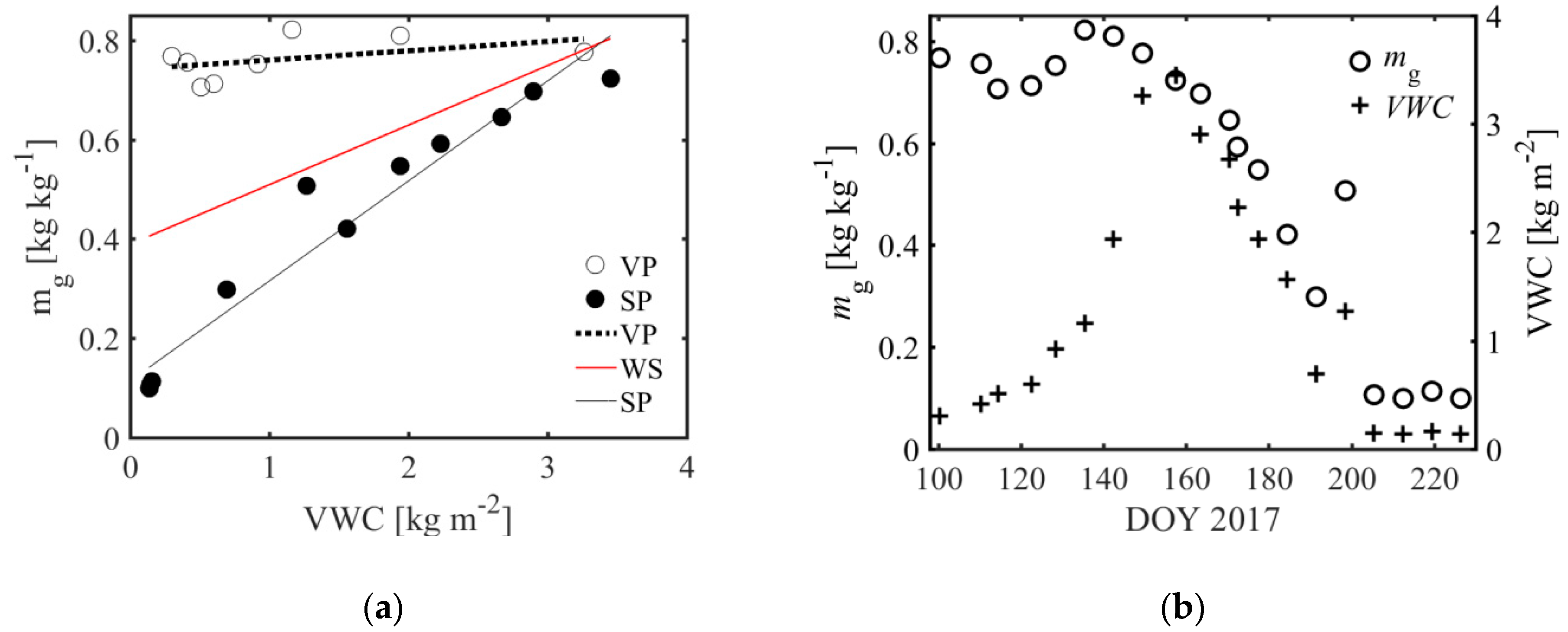
3.3. Comparison between m_g and VWC

Differences between gravimetric vegetation water content [kg kg⁻¹] and area-based VWC [kg m⁻²] were studied using linear regressions over the whole growing season, the vegetative growth stages (DOY ≤ 160), and the senescence stages after the peak vegetation water content (i.e., after flowering of the winter wheat; DOY > 160) (Figure 6a and

Table 4. Slope, intercept, and squared Pearson correlation coefficient (R²) of linear regression between in situ measured gravimetric vegetation water content (m_g) and the vegetation water content (VWC). Regressions were performed over the whole growing season, for only the growth stages (i.e., DOY ≤ 160), and for only the senescence stages (i.e., DOY > 160).

DOY.	Slope	Intercept	R2
Whole (100–226)	0.12	0.39	0.26
Growth (≤160)	0.02	0.74	0.21
Senescence (>160)	0.20	0.11	0.95

). In addition, the variation of the m_g and VWC over time is depicted (Figure 6b). The results show that for the whole growing season and the vegetative growth stages the correlation between m_g and VWC is rather low, with a R² of 0.26 and 0.21, respectively. This is related to the wheat growth where the VWC increases from values around 0.1 kg m⁻² to values around 3.5 kg m⁻² while m_g stays more or less constant during the same period with values around 0.75 (see Figure 6b). After crop flowering (i.e., DOY > 160) both the VWC and m_g show the same temporal behavior with decreasing values, as the vegetation starts to lose water during the senescence phase. This results in a high correlation between the m_g and VWC with a R² of 0.95 and slope and intercept values of 0.20 and 0.11. As expected, the VWC reflects the amount of water [kg] per unit area [m²], which is lowest during the beginning and the end of the growing season and highest during flowering. m_g on the contrary, is more closely describing the plant available water, which is high during the vegetative growth stages of the vegetation (i.e., no drought stress conditions were present with m_g ≥ 0.7) and low during senescence.

4. Discussion

This study represents a direct attempt to retrieve the gravimetric vegetation water content (m_g) under controlled conditions at the field scale over an entire growing season. The retrieved m_g values agree highly with the m_g reported by Grant et al. [18] for crop vegetation on global scale where m_g showed a mean and STD of 0.54 and 0.18, respectively. They used the effective medium approach [38,39] to estimate the m_g from L-band SMOS data. This approach calculates the canopy opacity (τ) based on a canopy structure coefficient, the wet biomass per area, the vegetation density, the wave number in air, the imaginary part of the vegetation dielectric constant, and the incidence angle [18,38]. Concerning the temporal evolution of our retrieved and in situ measured m_g, the study of Grant et al. [20] derived m_g from SMOS L-band optical depth (τ) values for the whole of 2010 over a coniferous forest in the U.S. and showed that the m_g values stay relatively constant over the year with values around 0.8. This confirms our finding that when the ratio between the water inside the plant and the wet biomass does not change (like during the vegetative growth stages), m_g is more or less unaffected because it directly represents this ratio. At the local scale, Wigneron et al. [37] found that m_g varied between 0.74 and 0.84 over the whole growing season (without the senescence stages) of a soy bean field. This is in good agreement to the findings of our study where m_g is generally stable during the vegetative growth stages of the winter wheat. Finally, on the basis of published reports about vegetation water content for different vegetation types (i.e., prairie grass, corn, soy beans, and others), Schmugge and Jackson [2] outlined that m_g varies between 0.6 and 0.8 for green vegetation, which was also the case in our study. Regarding the decrease of the retrieved and in situ measured m_g after DOY 160, such a behavior of m_g was also observed by Mätzler [40]. The author showed the temporal evolution of the dry matter fraction (m_d) over the whole growth cycle of an oat vegetation (with senescence stages included), which increased after the vegetation reached its highest VWC. This increase in m_d was caused by a decrease in VWC, where m_d reached a peak value of about 0.9 when the vegetation was fully senescent. Assuming that the m_g can be calculated from m_d (see Section 2.2.1), this study confirms our findings that the m_g can decrease after peaking of VWC to values around 0.1.

One unexpected result during our study was that our proposed approach underestimated m_g for the period between DOY 100 and 120 and overestimated m_g for DOY ≥ 180 in comparison to the in situ measured m_g. Indeed, when focusing on the δ parameter as the main reason for this behavior already small changes of δ result in relatively large changes in retrieved m_g (especially when the vegetation available water content was high) (see Figure 2 in Section 3.2). This was also confirmed by the study of Wigneron et al. [13] who observed that the δ of soy bean leaves had a distinct impact on the thermal emission especially for lower frequencies (i.e., L- and C-band). In addition, the study of Choe and Tsang [41] showed that for a cylindrical scatterer (i.e., stalk-dominated corn) changes of δ between 0.01% and 0.1% already led to significant changes in the measured emissivity at the L-band frequency. Hence, one possible solution to avoid these effects could be to use a daily variable δ or adapting δ according to the main phenological stages in the retrieval scheme. A daily variable δ was, for example, measured and retrieved by Wigneron et al. [37] over the whole growing season of a soy bean canopy where δ varied between 0.25 × 10⁻³ and 2.5 × 10⁻³. A daily variable δ could also be retrieved from the radar vegetation index, as suggested by Fink et al. [5]. Another reason for the underestimation and overestimation of m_g could have also been the assumptions made in the model of Ulaby and El-Rayes [3] (i.e., to assume a constant value for the temperature, salinity, and density of dry vegetation material (p = 0.33 g cm⁻³)), which were not able to describe the real conditions of the vegetation layer during the respective phenological stages. In this regard, Grant et al. [42], found a very small influence of temperature on ε_veg, but further tests are needed to investigate this option further.

Finally, to assume one static dielectric mixing model over the whole growing period of the winter wheat is also a strong simplification as the vegetation structure is actually changing (i.e., from a more leaf dominated vegetation in the beginning to a stronger stem-dominated vegetation during the main growing stages and the senescence phase). However, in our study it seems appropriate to describe the vegetation by the inclusion type which represents the dominant vegetation structure (i.e., the vn dielectric mixing model for the stalk-dominated wheat vegetation) as the linear regression between the retrieved and in situ measured m_g showed the closest fit to the optimum correlation line and a slightly smaller RMSE.

Future work will be directed towards further improving and validating the proposed m_g-retrieval approach by enabling a daily-varying or a phenology-adapted δ-retrieval. In addition, we will also investigate the possibility to analyze the relationship between the vegetation height and the δ-parameter allometrically, in order to have a dynamic δ along the growing season. Qin et al. [43], for example, studied the reproductive allocation of wheat plants for different growing densities and analyzed the relationship between the grain mass and vegetative mass by using an allometric function. They found a high correlation (i.e., R² > 0.9) between these two variables.

Moreover, the use of a more sophisticated objective function (i.e., not only using the squared difference between the measured and modelled τ as a decision criterion) could potentially improve the performance of the approach and could be investigated.

In addition, different τ-models, including polarization and/or angle-dependency on τ, could be tested (e.g., [32,44,45]). The τ-model of Schmugge and Jackson [2] was originally formulated to be used only with a nadir τ-parameter. Using a polarimetric τ for different incidence angles at the same time would certainly help to increase the accuracy of m_g retrievals and may also open the opportunity to use daily retrieved δ-parameters as mentioned above, since there would be more degrees of information [46,47]. At the moment we only use one polarization (i.e., V-polarization) and one incidence angle (i.e., 40°), which does not contain enough information to retrieve two variables simultaneously (i.e., m_g and δ) (see Section 2.2.1).

Concerning the potential of using our approach for other crop types and also at larger scales, it remains a subject of further research. We established controlled field conditions to investigate the different influences on τ and to develop an algorithm to extract m_g from τ. All the findings made during our study are only valid for winter wheat vegetation at a specific field and growing season.

Our recommendation for future studies would be to also use this attenuation-based approach for other crop types at the field scale and to continue the validation of the retrieved m_g with in situ measured m_g over longer observation periods and at different locations. Assessing the performance of our method at the regional or global scale is challenging due to limited availability of representative in situ validation data sets for m_g. In the event of having global coverage of radiometer-derived τ-values (e.g., estimated from SMOS or SMAP), LIDAR-based vegetation heights, and robust estimates for δ (e.g., radar-based as proposed by Fink et al. [5]), there might be an opportunity to use the proposed approach to generate global maps of m_g.

5. Summary and Conclusions

In this study, an approach was developed and applied to retrieve the gravimetric vegetation water content (m_g) of a winter wheat field over an entire growing season from L-band microwave radiometer observations (using V polarization data only). It is based on the inversion of a physical modeling framework describing the dependency of microwave radiation attenuation on vegetation height (d), vegetation volume fraction (δ), and m_g. The approach includes the Debye–Cole dual dispersion dielectric model of Ulaby and El-Rayes [3] as well as different vegetation dielectric mixing models [19]. The δ-parameter has a distinct impact on the microwave emission originating from the vegetation in the L-band and is another key variable for absorption inside the canopy [13]. We optimized δ to a constant value for this study, and analyze the impact of this assumption. The retrieved m_g agreed well with the in situ measured m_g (see Section 3.1). Their temporal agreement was high with a correlation of R² > 0.8. As expected, the vertical needles (vn) dielectric mixing model showed the best performance for the stalk-dominated wheat vegetation, with the closest fit of the linear regression to the optimum correlation line and a slightly smaller RMSE (see Figure 4 and Table 2 in Section 3.1).

In addition, the results implied that the assumption of a constant vegetation volume fraction (δ) over the growing season leads to an underestimation of m_g during the beginning of the vegetation growing phase and an overestimation of m_g during the senescence stage. To better understand this, a sensitivity analysis was performed on the m_g retrieval by varying the δ-input. It showed that small changes in δ already result in relatively large changes in retrieved m_g, especially when the actual water content within the vegetation is high. To improve the retrieval of m_g, δ could be defined on a daily basis or be adapted for dominant phenological stages (see Section 4). Additionally, no in situ measurements of δ or radar or LIDAR measurements (from which to estimate δ [5]) were available during the field experiment (see Section 2.2.1). However, results show that the assumption of a constant δ seems to be valid for the main growth stages of winter wheat (i.e., between DOY 120 and 180) (see Figure 4 in Section 3.1. and Figure 5 in Section 3.2).

Moreover, our comparison between gravimetric (m_g) and area-based (VWC) vegetation water content implied that m_g reflects the plant internal water content and is more closely related to the actual amount of water per unit of fresh biomass than VWC (see Figure 6 in Section 3.3). However, this finding cannot be generalized to a larger scale, as our experiment was only conducted at the field scale for a specific crop (winter wheat) and the results are therefore only valid for the presented data set. Still, results show that plant internal water is high during the growth stages of the vegetation and low during senescence. These results highlight that m_g is mainly the vegetation water content of the plants relative to their biomass amount. If both the biomass and the accompanying amount of water in the plant change (i.e., increase or decrease) at the same rate (such as, e.g., during the growing phase, for DOY 100-160), m_g does not change much, whereas VWC does increase due to the overall higher amount of water as a consequence of the higher biomass per area. When the biomass still continues to increase (or stays constant) and the VWC decreases (e.g., during the senescence phase, for DOY > 160), m_g begins to decrease as well.

We found that in situ measured structure parameters as vegetation height or biomass did not have a clear influence on m_g (results not shown). Concerning the influence of the dielectric mixing model on the m_g-retrieval, it was shown that it is appropriate to describe the vegetation over the whole growing season by the inclusion type which represents the dominant vegetation structure, i.e., vertical wheat stalks in our case. This corresponds to the vn mixing model.

References

1. Meyer, T.; Weihermüller, L.; Vereecken, H.; Jonard, F. Vegetation optical depth and soil moisture retrieved from L-band radiometry over the growth cycle of a winter wheat. Remote Sens. 2018, 10, 1637. [Google Scholar] [CrossRef]
2. Schmugge, T.J.; Jackson, T.J. A dielectric model of the vegetation effects on the microwave emission from soils. IEEE Trans. Geosci. Remote Sens. 1992, 30, 757–760. [Google Scholar] [CrossRef]
3. Ulaby, F.; El-Rayes, M. Microwave dielectric spectrum of vegetation—Part II: Dual-dispersion model. IEEE Trans. Geosci. Remote Sens. 1987, 5, 550–557. [Google Scholar] [CrossRef]
4. Yilmaz, M.T.; Hunt, E.R.; Goins, L.D.; Ustin, S.L.; Vanderbilt, V.C.; Jackson, T.J. Vegetation water content during SMEX04 from ground data and Landsat 5 thematic mapper imagery. Remote Sens. Environ. 2008, 112, 350–362. [Google Scholar] [CrossRef]
5. Fink, A.; Jagdhuber, T.; Piles, M.; Grant, J.; Baur, M.; Link, M.; Entekhabi, D. Estimating gravimetric moisture of vegetation using an attenuation-based multi-sensor approach. In Proceedings of the IEEE International Geoscience and Remote Sensing Symposium, Valencia, Spain, 22–27 July 2018; pp. 353–356. [Google Scholar]
6. Jackson, T.J.; Chen, D.; Cosh, M.; Li, F.; Anderson, M.; Walthall, C.; Doriaswamy, P.; Hunt, E.R. Vegetation water content mapping using Landsat data derived normalized difference water index for corn and soybeans. Remote Sens. Environ. 2004, 92, 475–482. [Google Scholar] [CrossRef]
7. Chen, D.; Huang, J.; Jackson, T.J. Vegetation water content estimation for corn and soybeans using spectral indices derived from MODIS near- and short-wave infrared bands. Remote Sens. Environ. 2005, 98, 225–236. [Google Scholar] [CrossRef]
8. Anderson, M.C.; Neale, C.M.U.; Li, F.; Norman, J.M.; Kustas, W.P.; Jayanthi, H.; Chavez, J. Upscaling ground observations of vegetation water content, canopy height, and leaf area index during SMEX02 using aircraft and Landsat imagery. Remote Sens. Environ. 2004, 92, 447–464. [Google Scholar] [CrossRef]
9. Saleh, K.; Wigneron, J.P.; Waldteufel, P.; de Rosnay, P.; Schwank, M.; Calvet, J.C.; Kerr, Y.H. Estimates of surface soil moisture under grass covers using L-band radiometry. Remote Sens. Environ. 2007, 109, 42–53. [Google Scholar] [CrossRef]
10. Wigneron, J.-P.; Chanzy, A.; Calvet, J.-C.; Bruguier, N. A simple algorithm to retrieve soil moisture and vegetation biomass using passive microwave measurements over crop fields. Remote Sens. Environ. 1995, 51, 331–341. [Google Scholar] [CrossRef]
11. Jackson, T.J.; Schmugge, T.J. Vegetation effects on the microwave emission of soils. Remote Sens. Environ. 1991, 36, 203–212. [Google Scholar] [CrossRef]
12. Wigneron, J.P.; Jackson, T.J.; O’Neill, P.; De Lannoy, G.; de Rosnay, P.; Walker, J.P.; Ferrazzoli, P.; Mironov, V.; Bircher, S.; Grant, J.P. Modelling the passive microwave signature from land surfaces: A review of recent results and application to the L-band SMOS & SMAP soil moisture retrieval algorithms. Remote Sens. Environ. 2017, 192, 238–262. [Google Scholar]
13. Wigneron, J.; Calvet, J.; Kerr, Y.; Chanzy, A.; Lopes, A. Microwave emission of vegetation: Sensitivity to leaf characteristics. IEEE Trans. Geosci. Remote Sens. 1993, 31, 716–726. [Google Scholar] [CrossRef]
14. Ulaby, F.T.; Jedlicka, R.P. Microwave dielectric properties of plant materials. IEEE Trans. Geosci. Remote Sens. 1984, 4, 406–415. [Google Scholar] [CrossRef]
15. O’Neill, P.; Chan, S.; Njoku, E.; Jackson, T.; Bindlish, R. Algorithm theoretical basis document (ATBD): Level 2 & 3 soil moisture (passive) data products. In Soil Moisture Active Passive (SMAP); Jet Propulsion Laboratory: Pesadena, CA, USA, 2015. [Google Scholar]
16. Kerr, Y.H.; Waldteufel, P.; Wigneron, J.-P.; Delwart, S.; Cabot, F.; Boutin, J.; Escorihuela, M.-J.; Font, J.; Reul, N.; Gruhier, C. The SMOS mission: New tool for monitoring key elements ofthe global water cycle. Proc. IEEE 2010, 98, 666–687. [Google Scholar] [CrossRef]
17. Entekhabi, D.; Njoku, E.G.; O’Neill, P.E.; Kellogg, K.H.; Crow, W.T.; Edelstein, W.N.; Entin, J.K.; Goodman, S.D.; Jackson, T.J.; Johnson, J. The soil moisture active passive (SMAP) mission. Proc. IEEE 2010, 98, 704–716. [Google Scholar] [CrossRef]
18. Grant, J.; Wigneron, J.; Williams, M.; Scholze, M.; Kerr, Y. Working towards a global-scale vegetation water product from SMOS optical depth. In Proceedings of the IEEE International Geoscience and Remote Sensing Symposium, Quebec City, QC, Canada, 13–18 July 2014; pp. 286–289. [Google Scholar]
19. Ulaby, F.T.; Long, D.G.; Blackwell, W.J.; Elachi, C.; Fung, A.K.; Ruf, C.; Sarabandi, K.; Zebker, H.A.; Van Zyl, J. Microwave Radar and Radiometric Remote Sensing; University of Michigan Press: Artech House, MI, USA, 2014. [Google Scholar]
20. Grant, J.P.; Wigneron, J.; Drusch, M.; Williams, M.; Law, B.E.; Novello, N.; Kerr, Y. Investigating temporal variations in vegetation water content derived from SMOS optical depth. In Proceedings of the IEEE International Geoscience and Remote Sensing Symposium, Munich, Germany, 22–27 July 2012; pp. 3331–3334. [Google Scholar]
21. Jonard, F.; Weihermuller, L.; Schwank, M.; Jadoon, K.Z.; Vereecken, H.; Lambot, S. Estimation of hydraulic properties of a sandy soil using ground-based active and passive microwave remote sensing. IEEE Trans. Geosci. Remote Sens. 2015, 53, 3095–3109. [Google Scholar] [CrossRef]
22. Polder, D.; van Santeen, J.H. The effective permeability of mixtures of solids. Physica 1946, 12, 257–271. [Google Scholar] [CrossRef]
23. Njoku, E.G.; Entekhabi, D. Passive microwave remote sensing of soil moisture. J. Hydrol. 1996, 184, 101–129. [Google Scholar] [CrossRef]
24. Li, L.; Gaiser, P.W.; Bo-Cai, G.; Bevilacqua, R.M.; Jackson, T.J.; Njoku, E.G.; Rudiger, C.; Calvet, J.-C.; Bindlish, R. WindSat global soil moisture retrieval and validation. IEEE Trans. Geosci. Remote Sens. 2010, 48, 2224–2241. [Google Scholar] [CrossRef]
25. Hunt, E.R.; Li, L.; Yilmaz, M.T.; Jackson, T.J. Comparison of vegetation water contents derived from shortwave-infrared and passive-microwave sensors over central Iowa. Remote Sens. Environ. 2011, 115, 2376–2383. [Google Scholar] [CrossRef]
26. Ulaby, F.; Wilson, E. Microwave attenuation properties of vegetation canopies. IEEE Trans. Geosci. Remote Sens. 1985, 5, 746–753. [Google Scholar] [CrossRef]
27. Brunfeldt, D.R.; Ulaby, F.T. Measured microwave emission and scattering in vegetation canopies. IEEE Trans. Geosci. Remote Sens. 1984, 6, 520–524. [Google Scholar] [CrossRef]
28. Grant, J.P.; Wigneron, J.P.; De Jeu, R.A.M.; Lawrence, H.; Mialon, A.; Richaume, P.; Al Bitar, A.; Drusch, M.; van Marle, M.J.E.; Kerr, Y. Comparison of SMOS and AMSR-E vegetation optical depth to four MODIS-based vegetation indices. Remote Sens. Environ. 2016, 172, 87–100. [Google Scholar] [CrossRef]
29. Kirdyashev, K.P.; Chukhlantsev, A.A.; Shutko, A.M. Microwave radiation of the earth’s surface in the presence of vegetation cover. Radio Eng. Electron. Phys. 1979, 24, 37–44. [Google Scholar]
30. Dirmeyer, P.A.; Gao, X.; Zhao, M.; Guo, Z.; Oki, T.; Hanasaki, N. GSWP-2: Multimodel analysis and implications for our perception of the land surface. Bull. Am. Meteorol. Soc. 2006, 87, 1381–1398. [Google Scholar] [CrossRef]
31. Shi, J.; Jackson, T.; Tao, J.; Du, J.; Bindlish, R.; Lu, L.; Chen, K.S. Microwave vegetation indices for short vegetation covers from satellite passive microwave sensor AMSR-E. Remote Sens. Environ. 2008, 112, 4285–4300. [Google Scholar] [CrossRef]
32. Wigneron, J.P.; Kerr, Y.; Waldteufel, P.; Saleh, K.; Escorihuela, M.J.; Richaume, P.; Ferrazzoli, P.; de Rosnay, P.; Gurney, R.; Calvet, J.C. L-band Microwave Emission of the Biosphere (L-MEB) model: Description and calibration against experimental data sets over crop fields. Remote Sens. Environ. 2007, 107, 639–655. [Google Scholar] [CrossRef]
33. Matzler, C. Microwave (1–100 GHz) dielectric model of leaves. IEEE Trans. Geosci. Remote Sens. 1994, 32, 947–949. [Google Scholar] [CrossRef]
34. Huyer, W.; Neumaier, A. Global optimization by multilevel coordinate search. J. Glob. Optim. 1999, 14, 331–355. [Google Scholar] [CrossRef]
35. Nelder, J.A.; Mead, R. A simplex method for function minimization. Comput. J. 1965, 7, 308–313. [Google Scholar] [CrossRef]
36. De Loor, G.P. Dielectric properties of heterogeneous mixtures with a polar constituent. Appl. Sci. Res. Sect. B 1964, 11, 310–320. [Google Scholar] [CrossRef]
37. Wigneron, J.-P.; Kerr, Y.; Chanzy, A.; Jin, Y.-Q. Inversion of surface parameters from passive microwave measurements over a soybean field. Remote Sens. Environ. 1993, 46, 61–72. [Google Scholar] [CrossRef]
38. Kerr, Y.H.; Njoku, E.G. A semiempirical model for interpreting microwave emission from semiarid land surfaces as seen from space. IEEE Trans. Geosci. Remote Sens. 1990, 28, 384–393. [Google Scholar] [CrossRef]
39. Wegmüller, U.; Mätzler, C.; Njoku, E.G. Canopy opacity models. In Passive Microwave Remote Sensing of Land-Atmosphere Interactions; VSP: Utrecht, The Netherlands, 1995. [Google Scholar]
40. Matzler, C. Seasonal evolution of microwave radiation from an oat field. Remote Sens. Environ. 1990, 31, 161–173. [Google Scholar] [CrossRef]
41. Tsang, L.; Choe, Y. A Mathematical Characterization of Vegetation Effect on Microwave Remote Sensing from the Earth; Texas A/M University, Remote Sensing Center: College Station, TX, USA, August 1983. [Google Scholar]
42. Grant, J.P. Global-scale Dynamic Monitoring of Vegetation Water Status for Improving Carbon Flux Estimates (VEGWAC); ESA STSE Final Report; Lund University: Lund, Sweden, 2016. [Google Scholar]
43. Qin, X.-L.; Weiner, J.; Qi, L.; Xiong, Y.-C.; Li, F.-M. Allometric analysis of the effects of density on reproductive allocation and harvest index in 6 varieties of wheat (Triticum). Field Crop. Res. 2013, 144, 162–166. [Google Scholar] [CrossRef]
44. Meesters, A.G.C.A.; De Jeu, R.A.M.; Owe, M. Analytical derivation of the vegetation optical depth from the microwave polarization difference index. IEEE Geosci. Remote Sens. Lett. 2005, 2, 121–123. [Google Scholar] [CrossRef]
45. Kurum, M.; O’Neill, P.E.; Lang, R.H.; Joseph, A.T.; Cosh, M.H.; Jackson, T.J. Effective tree scattering and opacity at L-band. Remote Sens. Environ. 2012, 118, 1–9. [Google Scholar] [CrossRef] [Green Version]
46. Konings, A.G.; McColl, K.A.; Piles, M.; Entekhabi, D. How many parameters can be maximally estimated from a set of measurements? IEEE Geosci. Remote Sens. Lett. 2015, 12, 1081–1085. [Google Scholar] [CrossRef]
47. Konings, A.G.; Piles, M.; Rötzer, K.; McColl, K.A.; Chan, S.K.; Entekhabi, D. Vegetation optical depth and scattering albedo retrieval using time series of dual-polarized L-band radiometer observations. Remote Sens. Environ. 2016, 172, 178–189. [Google Scholar] [CrossRef]
Figure 1. Experimental field setup (an aluminum bridge with ELBARA-II looking down toward the metal grid surface). (a) Vegetation conditions changing over the growing season of a winter wheat for selected phenological stages (be) at the Selhausen field laboratory (Germany) [1]. The experiment was conducted during a period of about 4 months from tillering of the winter wheat on April 10th (DOY 100) to the late senescence stage on August 14th 2017 (DOY 226).
Remotesensing 11 02353 g001
Figure 2. Conceptual scheme of the attenuation-based retrieval approach of the gravimetric vegetation water content (mg) based on radiometer-derived vegetation optical depth (τ) estimates (i.e., estimated from the brightness temperature (TB) measurements over a gridded plot using vertical polarization (p = V) [K], in situ measured vegetation height (d) [m], and a constant value for the vegetation volume fraction (δ) [–]. Different vegetation dielectric mixing models were used to derive the dielectric constant of the canopy (εcan), which was also used as an input for the τ model. Finally, mg was retrieved using the optimal (opt) vegetation dielectric constant (εveg) and based on the Ulaby and El-Rayes [3] model.
Remotesensing 11 02353 g002
Figure 3. Complex vegetation dielectric constant (εveg) retrievals for different mixing models (i.e., vertical needles (vn) (open and filled black squares) and random discs (rdi) (open and filled cyan diamonds)) using the proposed attenuation-based approach. These values are compared to εveg values (open and filled magenta triangles) derived from mg measurements. ε v e g denotes the real part and ε v e g the imaginary part of the dielectric constant.
Remotesensing 11 02353 g003
Figure 4. mg retrievals for different mixing models (i.e., vertical needles (vn) and random discs (rdi)) using the proposed attenuation-based approach. These values are compared to the in situ measured mg (ref) (a). In addition, the linear regressions between the retrieved mg parameters and the in situ measured mg for the vn (b) and rdi (c) case are shown. The open and closed black circles in the regression plots indicate the vegetative growth (DOY ≤ 160) and senescence stages (DOY > 160), respectively.
Remotesensing 11 02353 g004
Figure 5. Sensitivity analysis on the mg-retrieval by varying δ using the proposed attenuation-based approach. For this, two different vegetation dielectric mixing models were used, namely, the vertical needles (vn) (a) and random discs (rdi) (b) model. These results are compared to the in situ measured mg (ref). Note that the black circles represent the δ-value, which leads to the closest fit between the retrieved and in situ measured mg.
Remotesensing 11 02353 g005
Figure 6. Linear regressions between the in situ measured gravimetric vegetation water content (mg) [kg kg−1] and the area-based vegetation water content (VWC) [kg m−2] for the whole growing season (WS)(open and filled black circles and red solid line), for only the vegetative growth phase (VP) (i.e., DOY < 160) (open black circles and dotted line), and for only the senescence phase (SP) (i.e., DOY > 160) (filled black circles and solid line) (a). In situ measured mg and VWC over time (b).
Remotesensing 11 02353 g006