Ground Truth Validation of Sentinel-2 Data Using Mobile Wireless Ad Hoc Sensor Networks (MWSN) in Vegetation Stands

Abstract

Satellite-based remote sensing (RS) data are increasingly used to map and monitor local, regional, and global environmental phenomena and processes. Although the availability of RS data has improved significantly, especially in recent years, operational applications to derive value-added information products are still limited by close-range validation and verification deficits. This is mainly due to the gap between standardized and sufficiently available close-range and RS data in type, quality, and quantity. However, to ensure the best possible linkage of close-range and RS data, it makes sense to simultaneously record close-range data in addition to the availability of environmental models. This critical gap is filled by the presented mobile wireless ad hoc sensor network (MWSN) concept, which records sufficient close-range data automatically and in a standardized way, even at local and regional levels. This paper presents a field study conducted as part of the Durable Environmental Multidisciplinary Monitoring Information Network (DEMMIN), focusing on the information gained with respect to estimating the vegetation state with the help of multispectral data by simultaneous observation of an MWSN during a Sentinel-2A (S2A) overflight. Based on a cross-calibration of the two systems, a comparable spectral characteristic of the data sets could be achieved. Building upon this, an analysis of the data regarding the influence of solar altitude, test side topography and land cover, and sub-pixel heterogeneity was accomplished. In particular, variations due to spatial heterogeneity and dynamics in the diurnal cycle show to what extent such complementary measurement systems can improve the data from RS products concerning the vegetation type and atmospheric conditions.

1. Introduction

The Copernicus initiative is aimed at developing a European geo-information market. The Copernicus program is primarily concerned with implementing environment and security-related information services based on observation data received from Earth observation (EO) satellites in the interplay with ground-based information [1]. In particular, the Sentinel-2 (S2) mission [2], which can be considered a complement to the Landsat mission [3], focuses on long-term environmental monitoring. One of the key problems in recent environmental monitoring is the gap in temporal and spatial scales between measurement and management [4]. To adequately describe ecosystem conditions, information from different data sources is needed: spatial information from EO satellites and temporal high-resolution and continuous measurements via ground-based measurement networks to capture dynamic processes and local spatial heterogeneity. As part of the focus of national and European terrestrial long-term monitoring initiatives (e.g., [5,6,7]), agencies such as the German Aerospace Center operate different scientific data pools to guarantee the scientific community simplified and cost-effective or cost-free access to remote sensing (RS) data, for instance, the LANDSAT 7/ETM+ Scientific Data Pool or the TerraSAR-X Scientific Data Pool (https://sss.terrasar-x.dlr.de; accessed on 18 September 2023).

Since remote sensors record the amount of electromagnetic radiance at the sensor in different wavebands, the measured radiance represents the traits of abiotic and biotic surfaces from which the radiance emanates [8]. RS technology can only record entities of vegetation health and states based on physical characteristics, as well as the reflectance and scattering properties of individual plants, communities, habitats, and biomes [8,9], whereby only the superpositions of plant processes and signals (a composite of spectral features) become visible in EO satellite data. Therefore, ground-based measurements are necessary to detect changes locally with comparable spectral sensor characteristics in high temporal and spatial resolutions. The appropriate data can be made available partially by close-range measurements [10], which measure close-range data parallel to overpasses of satellite-based RS systems. However, an adaptive ground-based reference system can be useful for adequate close-range calibration and validation due to the

• Heterogeneity and diversity of the land cover;
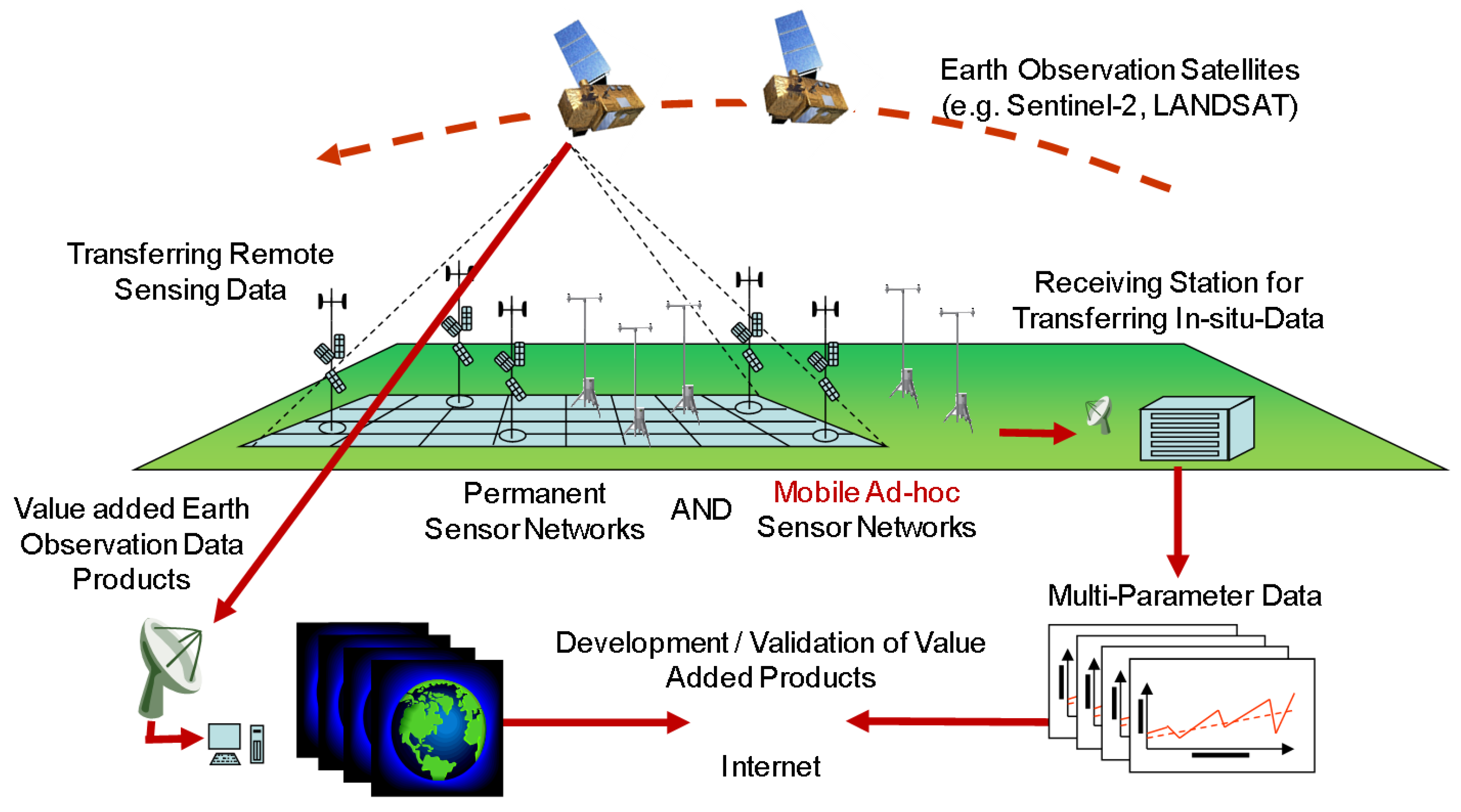
• Existing structural gaps within stationary measurement networks, which can be supported temporarily by supplementing and complementing measuring systems for special investigations;
• The differences in spectral and geometric requirements of various RS systems.

Those adaptive ground-based reference systems can be designed and developed as mobile wireless ad hoc sensor networks (MWSN), which are a promising application for a satisfactory solution in the ground-truthing of superspectral RS data [11,12]. Such systems (cf. Section 2.3.1) serve a short-term campaign-oriented deployment. Due to the relatively compact design and automated data acquisition and network topology, agile deployment in the field and spontaneous adjustment of the measurement design, similar to a mobile measuring device, are possible. These have already been successfully tested for identifying the main drivers of the seasonal decline of near-infrared reflectance of a temperate deciduous forest [13] and validating other RS systems, such as Cosmic-Ray Neutron Sensors [14,15]. For EO satellites, field deployment of the sensor nodes supports a comprehensible field of view (FOV) and allows for adjustment of the sensor technology based on temporal resolution (e.g., Nyquist sampling theorem) or sensor types depending on the biotic process. Significantly, the improvement of atmospheric corrections and resampling algorithms of single multispectral channels or derived vegetation indices hold great potential for the data quality management of RS value-added products.

Mobile monitoring is increasingly used as a complementary tool to capture environmental properties with high spatial resolution and to gain insights into spatial variability, which a stationary network could not enable [16,17,18]. This complementary monitoring requires careful setup with a sufficient number of replicates in terms of desired reliability and spatial resolution [16], with stationary devices being able to collect data over a time period at a specific location in the network, while mobile devices can collect data over large geographic regions [18] as well as in plot-scale setups. While a variety of monitoring applications (monitoring of, e.g., air quality, traffic, urban heat islands) take advantage of the joint application of stationary and mobile measurement systems [16,17,18,19,20], their use is still relatively seldom in the field of RS data validation.

Figure 1 illustrates the complementary interaction of terrestrial close-range measurement methods and RS technologies in providing spatially and temporally high-resolution data sets, which are thematically detailed, for diverse applications. Here, the close-range system offers a setup for detecting a homogeneous land cover class which minimizes the influence of spectral mixture on the pixels. The combination of both sensing technologies enables users’ requirements for information. This highlights that RS and close-range data acquisitions are an indispensable part of the modern exploration of the Earth and that there is a need to develop models for the aggregation of data with different origins.

Since the use of RS is subject to environmental aspects, the determination and monitoring of biomass above ground represents one of the most critical objectives [22,23]. In this context, determining the type and composition of vegetation and assessing its quantity and/or quality is the focus of interest.

Based on vegetation indices, different environmental parameters can be computed, e.g., canopy cover [24], leaf area index (LAI) [25,26,27], interception storage [28], surface temperature [29,30], air temperature [31], the canopy structure and photosynthesis of different vegetation types (e.g., [32]), the fraction of absorbed photosynthetically active radiation [33], crop identification and yield estimation (e.g., [34,35]), plant diseases [36], and proxies to derive soil characteristics and soil moisture [37,38].

Although these studies demonstrated the usability of vegetation indices to derive diverse environmental parameters, Vermote and Vermeulen [39] and Mannschatz et al. [40] discussed some uncertainties in estimating vegetation indices. They showed that, e.g., different parameterizations of atmospheric correction can lead to different LAI values when related to the normalized difference vegetation index (NDVI), which serves as an indicator for describing biomass development and vegetation activity, even when using the same data set. Different vegetation indices were developed considering the different influencing factors such as atmospheric influences or soil background. Therefore, different indices have been developed for minimizing influencing factors such as atmospheric effects or soil background (see, e.g., Gong et al. [41] or Viña et al. [27] for more information).

Against this backdrop, ensuring the quality of intended Copernicus information services based on, e.g., the S2 data, as well as protecting data integrity (i.e., ensuring the accuracy and consistency of the S2 data and derived information) is thus an urgent task to be resolved. This task can only be accomplished by validating the S2 data through the simultaneous provision of close-range and in situ data.

This paper discusses the use of an adaptable MWSN designed for assisting RS missions, such as S2, as the completion of existing stationary monitoring networks. Furthermore, we want to provide guidelines for the validation of the S2 data by MWSNs to develop value-added products with error logs, e.g., monitoring sensible environmental parameters and providing an outlook for other EO missions.

2. Material and Methods

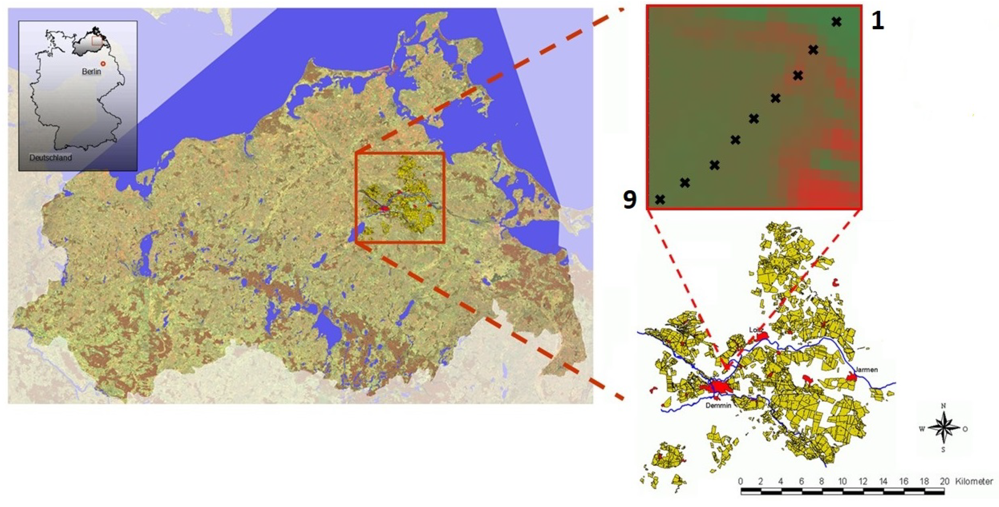
2.1. DEMMIN Validation Test Site

The calibration and validation site DEMMIN is located in Mecklenburg-Western Pomerania, Germany. DEMMIN was designed with particular attention to the test site requirements necessitated by the broadest possible range of uses of operational RS applications. In addition, this site was included in the TERENO initiative [6] to develop a platform to address technical and technological developments related to RS for monitoring from an environmental and climate perspective. The TERENO initiative aims to create observation platforms based on an interdisciplinary and long-term research program with close cooperation between several German institutions to study the consequences of global change for terrestrial ecosystems, their complex feedback mechanisms, and the socio-economic impacts [4,6,42,43]. The intention is to provide a long-term series of system variables for analyzing and predicting the consequences of global change based on integrated model systems, which will be used to derive efficient mitigation and adaptation strategies based on remote sensing data and in situ measurement networks. As an environmental monitoring network, the DEMMIN test site operates more than 40 measurement stations with scientific instruments for measuring atmospheric and soil parameters. Although, several parameters are collected automatically, some, such as spectrometric signatures, require regular field campaigns [44].

The site extends from ${54}^{°}{2}^{\prime }{54.29}^{″}$N, ${12}^{°}{52}^{\prime }{17.98}^{″}$E to ${53}^{°}{45}^{\prime }{40.4}^{″}$N, ${13}^{°}{27}^{\prime }{49.4}^{″}$E, according to Gerighausen et al. [45]. Figure 2 shows a part of the site where an MWSN was installed as a transect (northeast to southwest) in the headland and in a canola field (marked as black crosses) with increasing distance from the branch of the Peene River.

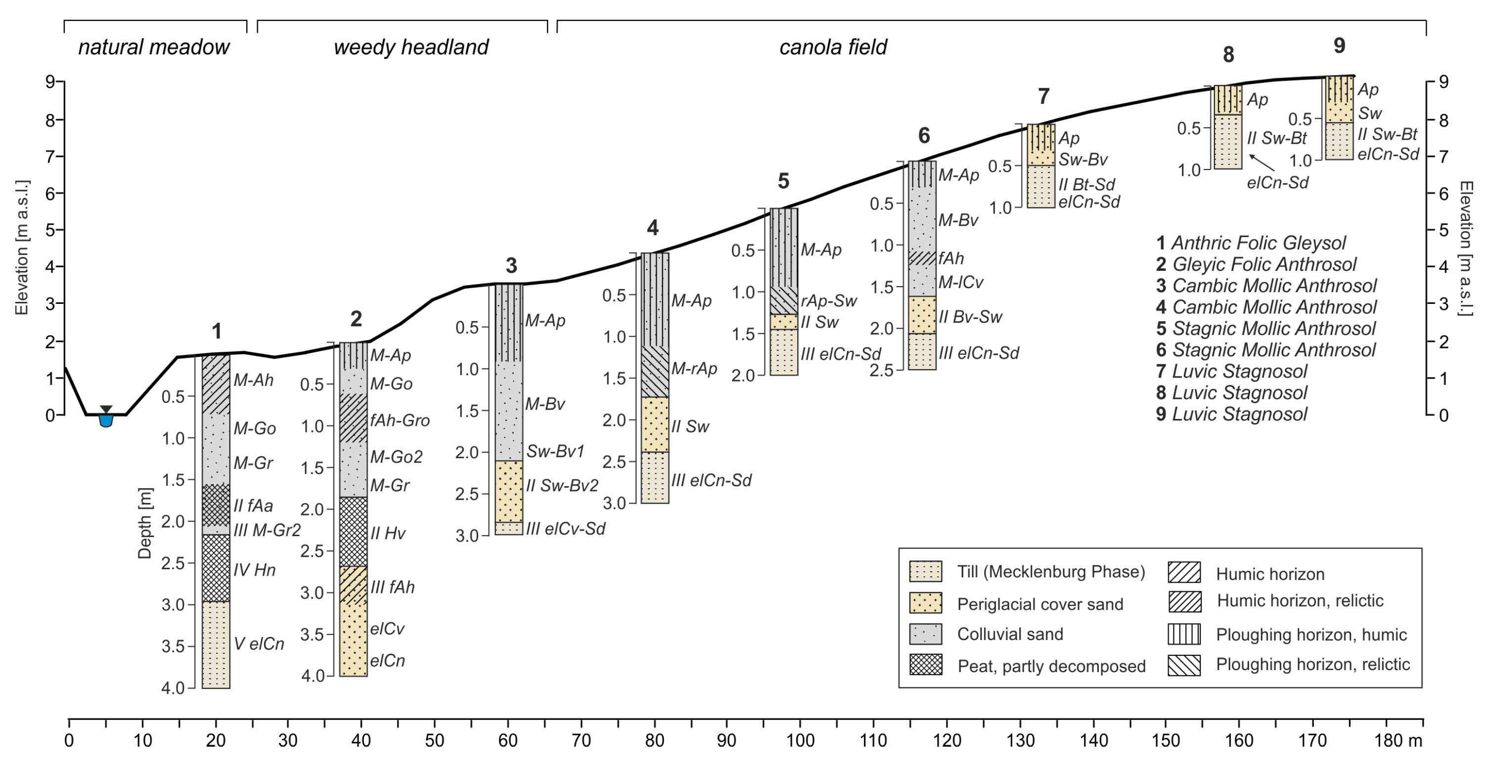
2.2. Soil and Vegetation Characteristics

Along the MWSN measurement transect, a succession of nine soil profiles was investigated using sediment cores with an 8 cm diameter (Figure 3). Adjacent to the measuring devices, the drillings follow a straight line down the hill to a creek, which is a tributary of the Peene River. The investigation area is part of the Western Pomeranian till plains, originating from the youngest glacial advance of the Weichselian glaciation. Diamictic tills rich in carbonate and periglacial cover sands form the parental material for soil development.

While the upper Positions 7–9 represent strongly eroded soils, the mid- and down-slope Positions 1–6 show thick colluvial covers due to plowing and soil erosion (Figure 3). The vegetation cover at Position 1 (natural meadow) was well supplied with water, very closed, and fully developed (Figure 4a). The vegetation at Position 2 was a weedy meadow used as a driveway and headland by farmers and showed firmly compacted upper soils. Position 3 represents a transient area from the meadow to the canola field, standing likewise in the range of the headland (Figure 4b). Starting from Position 4, all other measuring stations were placed in the canola field (a sample is given in Figure 4c). The observed distribution of vegetation or land use and soil genesis is also reflected in the corresponding soil types and humus contents (see

Table 1. Topsoil sediment characteristics and the organic content of nine soil profiles along the MWSN measurement transect.

Profile	Topsoil Sediment	Organic Content
1	slightly loamy sand	(2–4%)
2	slightly loamy sand with fine and medium gravel	(<1%)
3	slightly silty sand	(<1%)
4	medium sand, slightly silty sand	(<1%)
5	medium sand with fine sand, fine gravel, and medium gravel	(<1%)
6	slightly silty sand with fine and medium gravel	(<1%)
7	slightly silty sand with fine gravel	(<1%)
8	moderately silty sand	(<1%)
9	moderately loamy sand	(<1%)

), which influence the related plant growth and, thereby, indirectly, the temporal development of, e.g., vegetation indices.

2.3. Close-Range Data and Remote Sensing Data

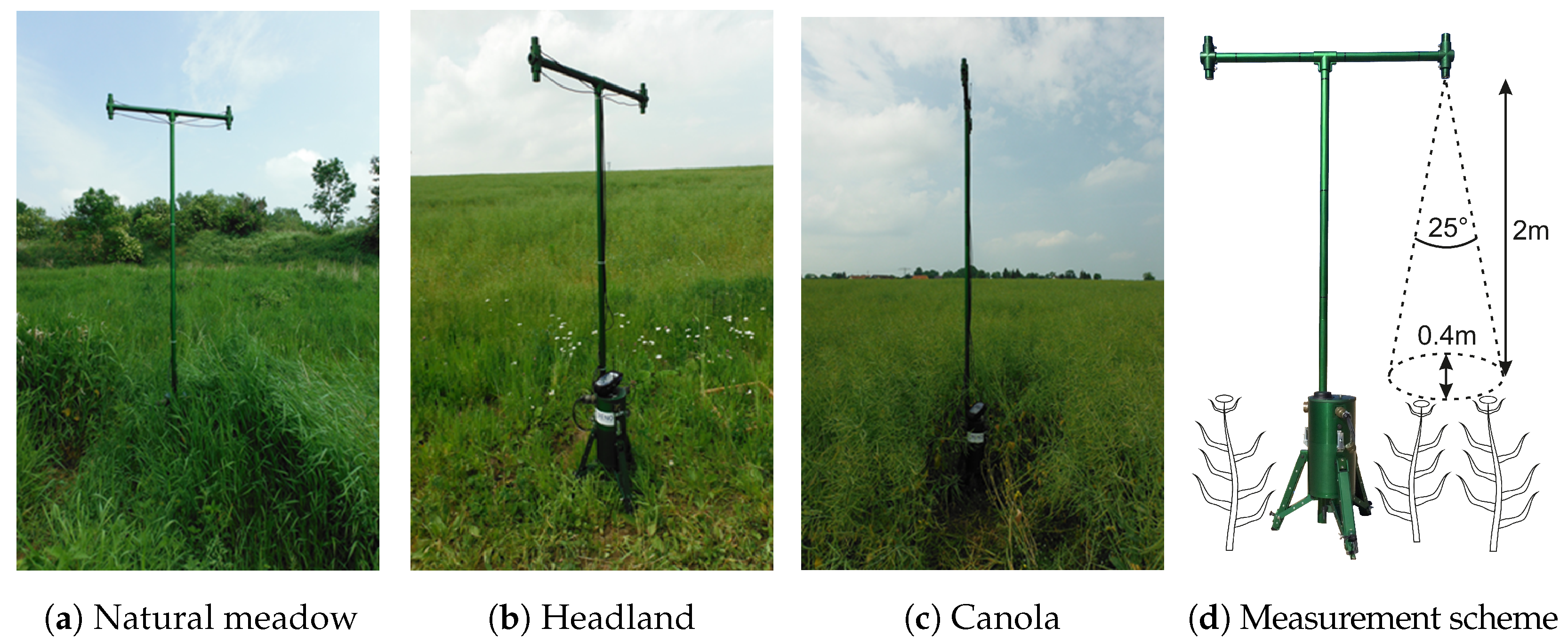
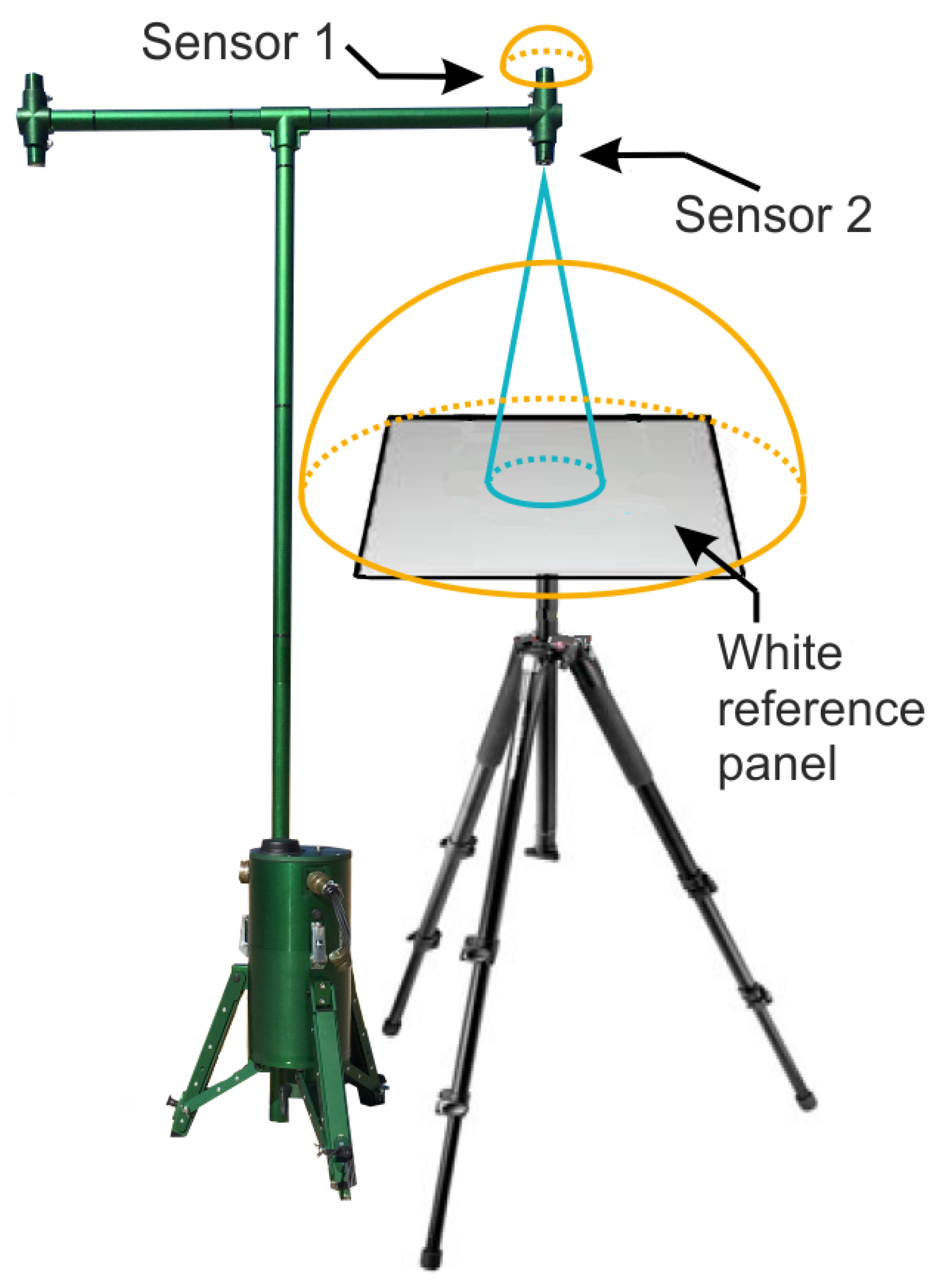
2.3.1. Mobile Wireless Ad Hoc Sensor Network

The presented MWSN is a joint development of the Helmholtz Centre for Environmental Research—UFZ, the Institut für Mikroelektronik- und Mechatronik-Systeme gemeinnützige GmbH (IMMS), and the Kompass GmbH. Further information regarding the network protocol and other applications can be found in Götze et al. [47] and Töpfer et al. [48].

The deployed network uses a wireless low-power protocol [49,50], which forms the basis of the proprietary protocol and modular sensor platform of the MWSN, respectively, previously developed at IMMS [47]. The Simple Network Time Protocol is used for time synchronization [51], which provides accuracies from 1 ms to 50 ms for most applications, depending on the characteristics of the synchronization source and the network paths [51]. In establishing and maintaining their network without the need for specialist operators, the MWSN offer also features self-organizing behavior [52]. In conclusion, inserting or removing sensor nodes from the network is an automated process with no significant effort. In addition, the systems have an integrated power supply, which allows them to carry out their measurement procedure autonomously in the field and send the corresponding data wirelessly.

To validate the S2 data, nine MWSN nodes were installed along the measurement transect on the DEMMIN test side. Figure 4d exemplarily shows an autonomous MWSN node for measuring four multispectral wavebands comparatively to specific S2A wavebands (see Table 2), allowing the detection of particular parameters for vegetation, e.g., the NDVI. The corresponding multispectral sensors (MSH-OS-NB-500HWB-IP67) are distributed by Kompass GmbH, headquartered in Ilmenau, Germany. The multispectral sensors are designed with removable sensor heads to allow the appropriate interference filters to be changed. The advantage of this version is that the spectral characteristics of the sensors can be adjusted to specific satellite missions or vegetation indices, among other things. Interference filters available on the market were used for this purpose. Producing separately mountable filters with the same spectral transmission curve is technically very difficult to realize and cost-intensive. Therefore, certain tolerances regarding a filter’s central wavelength and bandwidth (see Table 2) are expected for its production. However, cross-calibration methods can compensate for these deviations (see Section 2.4.2). The sampling rate for the measurement campaign was set to one capture per 300 s. Specific tolerances are expected concerning the long-term stability of the sensors, too. Many manufacturers (using similar components and materials to produce devices such as the MWSN sensors) indicate a long-term sensitivity degradation of 2% annually [53]. However, Akitsu et al. [53] observed an annual degradation of up to 11%, depending on the climatic conditions and sensor type, for a selection of commercially available products. Therefore, calibration after each measurement campaign, each filter change, and at least once a year is also recommended for the MWSN sensors.

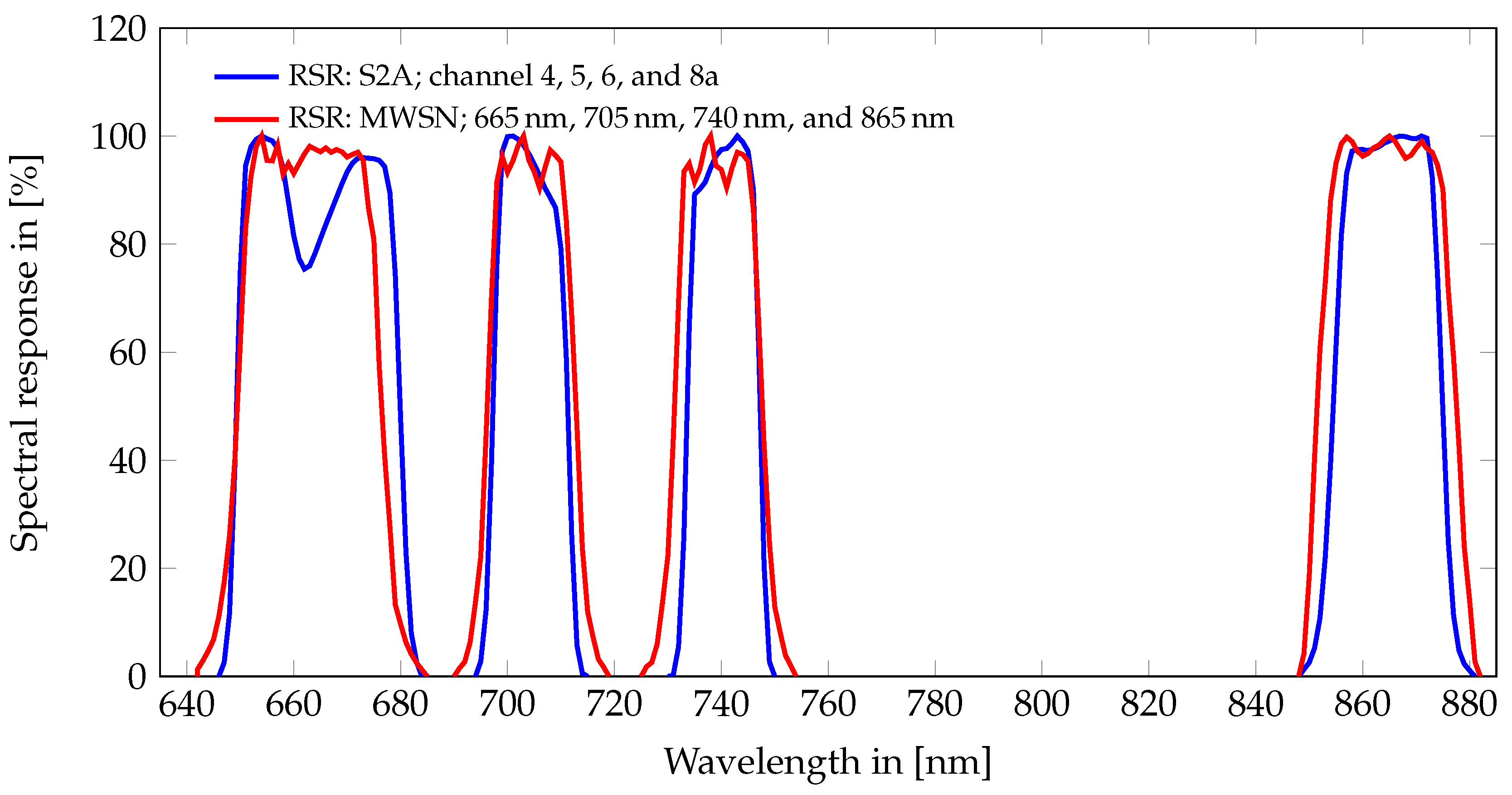
2.3.2. Sentinel-2 Data

The S2 mission consists of two satellites (S2A—launch: 23 June 2015, S2B—launch: 7 March 2017) in the same sun-synchronous orbit. The mission is considered a supplement and continuation of the Landsat or SPOT missions and will deliver continuous multi-spectral RS data [54,55]. The S2 data are mainly used to record and monitor vegetation, soil, and water [56]. The spatial, radiometric, and spectral sensor characteristics of S2 are given in Table 2.

Table 2. The spatial and spectral characteristics of S2A data (https://sentinels.copernicus.eu/web/sentinel/technical-guides/sentinel-2-msi/msi-instrument; accessed on 18 September 2023) complemented by the MWSN sensors.

Band Number (S2A/MWSN)	Central Wavelength S2A (nm)	Channel Bandwidth (FWHM) S2A (nm)	Central Wavelength MWSN (nm)	Channel Bandwidth (FWHM) MWSN (nm)	Spatial Resolution S2A (m)
4/1	$664.6$	30	$665\pm 3$	$25\pm 5$	10
5/2	$704.1$	14	$705\pm 3$	$20\pm 3$	20
6/3	$740.5$	14	$740\pm 3$	$20\pm 3$	20
8a/4	$864.7$	21	$865\pm 3$	$25\pm 3$	20

Table 2. The spatial and spectral characteristics of S2A data (https://sentinels.copernicus.eu/web/sentinel/technical-guides/sentinel-2-msi/msi-instrument; accessed on 18 September 2023) complemented by the MWSN sensors.

Band Number (S2A/MWSN)	Central Wavelength S2A (nm)	Channel Bandwidth (FWHM) S2A (nm)	Central Wavelength MWSN (nm)	Channel Bandwidth (FWHM) MWSN (nm)	Spatial Resolution S2A (m)
4/1	$664.6$	30	$665\pm 3$	$25\pm 5$	10
5/2	$704.1$	14	$705\pm 3$	$20\pm 3$	20
6/3	$740.5$	14	$740\pm 3$	$20\pm 3$	20
8a/4	$864.7$	21	$865\pm 3$	$25\pm 3$	20

The validation campaign was planned from 27 May 2016 to 19 June 2016. The relatively short measurement campaign is a general problem of mobile ground-based observation of land used for agricultural purposes. Representative plots are usually limited to long-term observation. In this case, this farmland was conventionally cultivated. Therefore, such a campaign depends on tenants’ approval, who understandably can only permit finite investigation periods to maintain operational processes, such as soil tillage or crop protection applications.

Unfortunately, only one evaluable S2 acquisition covered the test site during the campaign period on 11 June (see

Table 3. Available data: data recording by S2 and LANDSAT-8 during the validation campaign from 27 May 2016 to 19 June 2016.

Satellite Data	Data Recording	Usability	Comment
S2A L1C	29 May 2016	no	cloudy (≥40% coverage) and the transect is not covered by the scene
S2A L1C	8 June 2016	no	the transect is not covered by the scene
S2A L1C	11 June 2016	yes	these data are used in the manuscript
S2A L1C	18 June 2016	no	cloudy (≥50% coverage) and the transect is not covered by the scene
LANDSAT-8 L1	30 May 2016	no	haze over the transect
LANDSAT-8 L1	6 June 2016	yes	not comparable to S2A (different angles of view cause different spectral information due to BRDF effects)
LANDSAT-8 L1	18 June 2016	no	cloudy (≥40% coverage)

). The full L1C-Granule (Level-1C: top of atmosphere reflectance in cartographic geometry) was covered by clouds in about 11% of its area. However, the test area itself was free of clouds and cloud shadows.

Considerations to evaluate comparable data from other missions such as LANDSAT-8, which, in principle, would be technically possible with a cross-calibration of the systems, were not pursued because the spectral characteristics of the sensors of the MWSN have been designed explicitly for S2. Therefore, the primary goal is to validate exactly these data. However, in the example of LANDSAT-8, only a further recording of data would be suitable (see Table 3). In addition, the bidirectional reflectance distribution function (BRDF) effects lead to other uncertainties due to the different viewing angles of the sensors of S2 and LANDSAT-8. An accurate quantification would only be possible with an adapted radiative transfer model for the vegetation stands, which is beyond the scope of this publication. The presented work seeks to address how to implement MWSN technology in future monitoring strategies and campaigns and enable such further analysis.

2.4. Pre-Processing of Remote Sensing Data

2.4.1. Geo-Correction and Atmospheric Correction

The pre-processing of the S2 data includes a geometric and atmospheric correction to allow quantitative data processing. After that, the reflectance spectra of the S2A scene for all nine positions were extracted and compared with close-range data by the MWSN.

Atmospheric correction of S2A data on 11 June 2016 (granule: T33UUV) was performed using the ESA L2A-processor Sen2Cor (Level-2A: bottom of atmosphere reflectance in cartographic geometry) version 2.9 since there are no L2A data from 2016 in the current ESA archive. The processor was running with the default configuration: rural aerosols, variable visibility, midlatitude summer atmospheric profile, water vapor correction, ozone content from the metadata, no cirrus correction, no BRDF correction, adjacency range of 1000 m, and flat terrain at an altitude of 10 m.

2.4.2. Sensor System Cross-Calibration

For a quantitative analysis of different RS sensors, the devices must be on a consistent radiometric calibration scale [57]. Cross-calibration is the only viable solution to tie similar and differing sensors into a standard radiometric scale [58]. For an ideal cross-calibration, the two sensors should observe the same target simultaneously with the same viewing geometry [59]. Since, in this measurement design, the different viewing geometries are part of the investigations, only the internal spectral characteristics of the sensor systems were considered for the calibration. These differences in spectral responses between the opto-electronic sensors lead to a systematic waveband offset when comparing these sensors, as the two sensors respond differently to the same electromagnetic source [58,60].

To apply this calibration between S2 and the sensor network channels, a spectral band adjustment factor (SBAF) was calculated for each waveband. The transfer coefficients for S2A ($T{C}_S$) and the MWSN ($T{C}_W$) were determined by the respective convolution of the relative spectral responses (RSR) with the solar spectrum ($E_0$) derived by Thuillier et al. [61] for each band instead of a hyperspectral profile. The relative spectral responses for the close-range sensor channels were provided by the manufacturer in 1 nm spectral resolution (supplied datasheet). The corresponding data for S2A are given by the European Space Agency [62].

$$T{C}_W=\frac{{\int }_{{\lambda }_1}^{{\lambda }_2}{E}_{0}RS{R}_{W}d\lambda }{{\int }_{{\lambda }_1}^{{\lambda }_2}RS{R}_{W}d\lambda }$$

(1)

$$T{C}_S=\frac{{\int }_{{\lambda }_1}^{{\lambda }_2}{E}_{0}RS{R}_{S}d\lambda }{{\int }_{{\lambda }_1}^{{\lambda }_2}RS{R}_{S}d\lambda }$$

(2)

$$SABF=\frac{T{C}_W}{T{C}_S}$$

(3)

where ${\lambda }_1$ and ${\lambda }_2$ are the limits (RSR $<1\%$) of the multispectral bands.

Once the band-specific spectral band adjustment factors are calculated, the sensor reflectances of the MWSN ($R_{\lambda }$) can be divided by these factors to adjust the spectral response differences between the two sensors.

$${\overline{R}}_{\lambda }=\frac{R_{\lambda }}{SABF}$$

(4)

2.4.3. Inter-Calibration of the Close-Range Sensors

Usually, light-sensor calibration is performed by sensor manufacturers or professional laboratories because this type of calibration is time-consuming, expensive, and disruptive to measurements since the sensors have to be dismounted, gathered from field sites, and delivered back and forth [63]. Since the MWSN aims to deploy event-based sensor nodes with possibly adapted spectral characteristics in the study area, an inter-calibration is provided by an accurate and straightforward in situ calibration method based on relative sensitivities described by Jin and Eklundh [63]. This user-level method for sensor pairs in daylight estimates bi-hemispherical reflectance or hemispherical–conical reflectance, suitable for multispectral sensors.

To perform the inter-calibration, a test rig was built as a free field test according to the description of Jin and Eklundh [63] for the close-range calibration of light sensors with hemispherical–conical sensor pairs (see Figure 5). The measurements were applied over ten days with a sampling rate of 10 s to achieve a high calibration accuracy in accordance with the calibration procedures proposed by Jin and Eklundh [63]. The procedure assumes that the light Sensor 1, with an ideal angular response, is oriented upwards to measure incoming solar radiation. The incident radiant flux density, depending on the sun’s zenith angle and azimuth angle, has a diffuse and a direct fraction. For the downward-looking conical-FOV Sensor 2, a white reference panel is placed horizontally in the sensor nadir direction, which may be viewed together with Sensor 2 as an upward-oriented sensor system that measures irradiance. By neglecting the nearby ground reflection, the sensor pair being inter-calibrated measures the same irradiance quantity as the sensor readings. Using linear regression for the two time series, the sensitivity ratio can be determined and used as a correction factor for the calculation of the reflectance.

2.4.4. Vegetation Indices

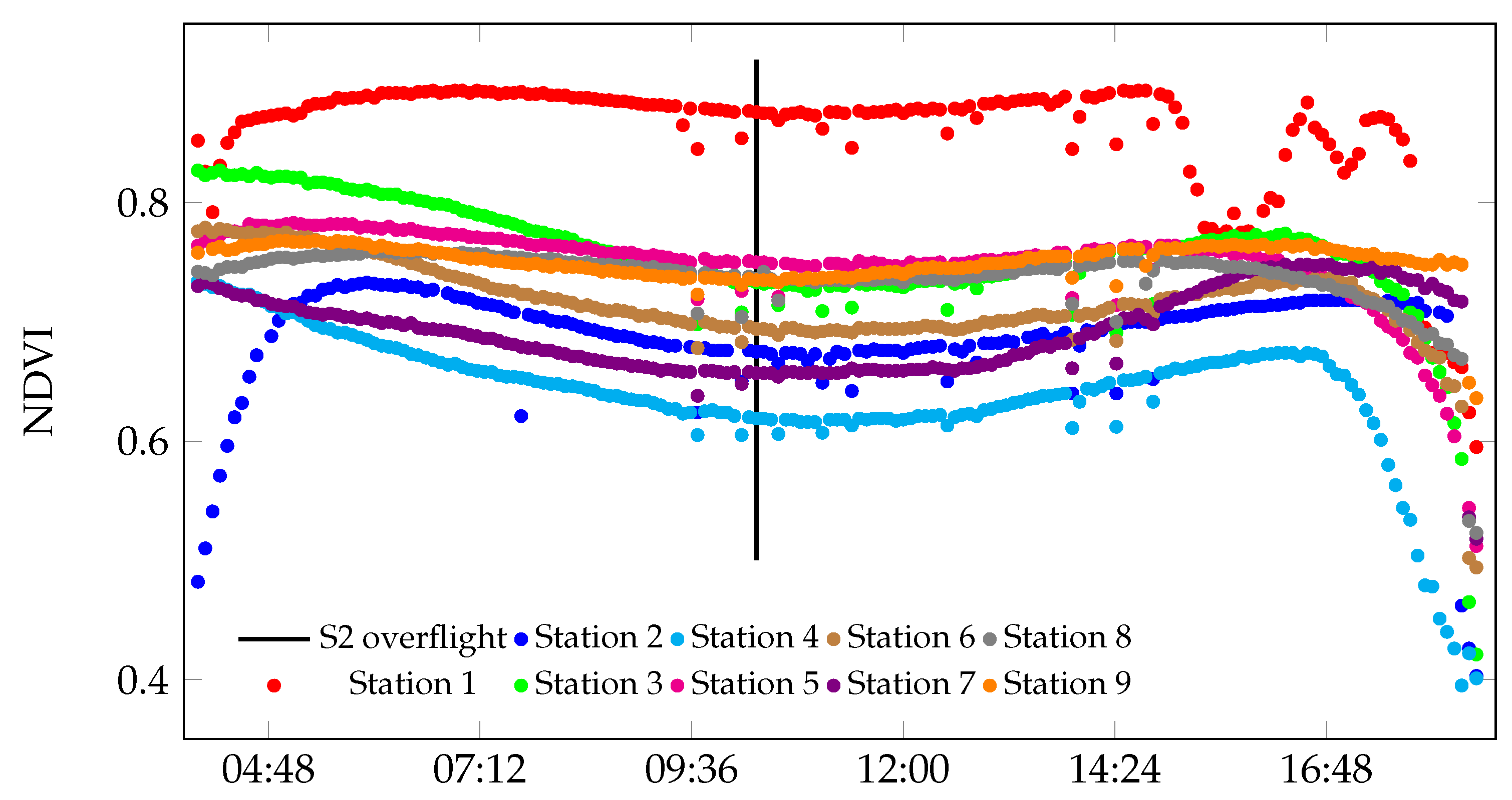
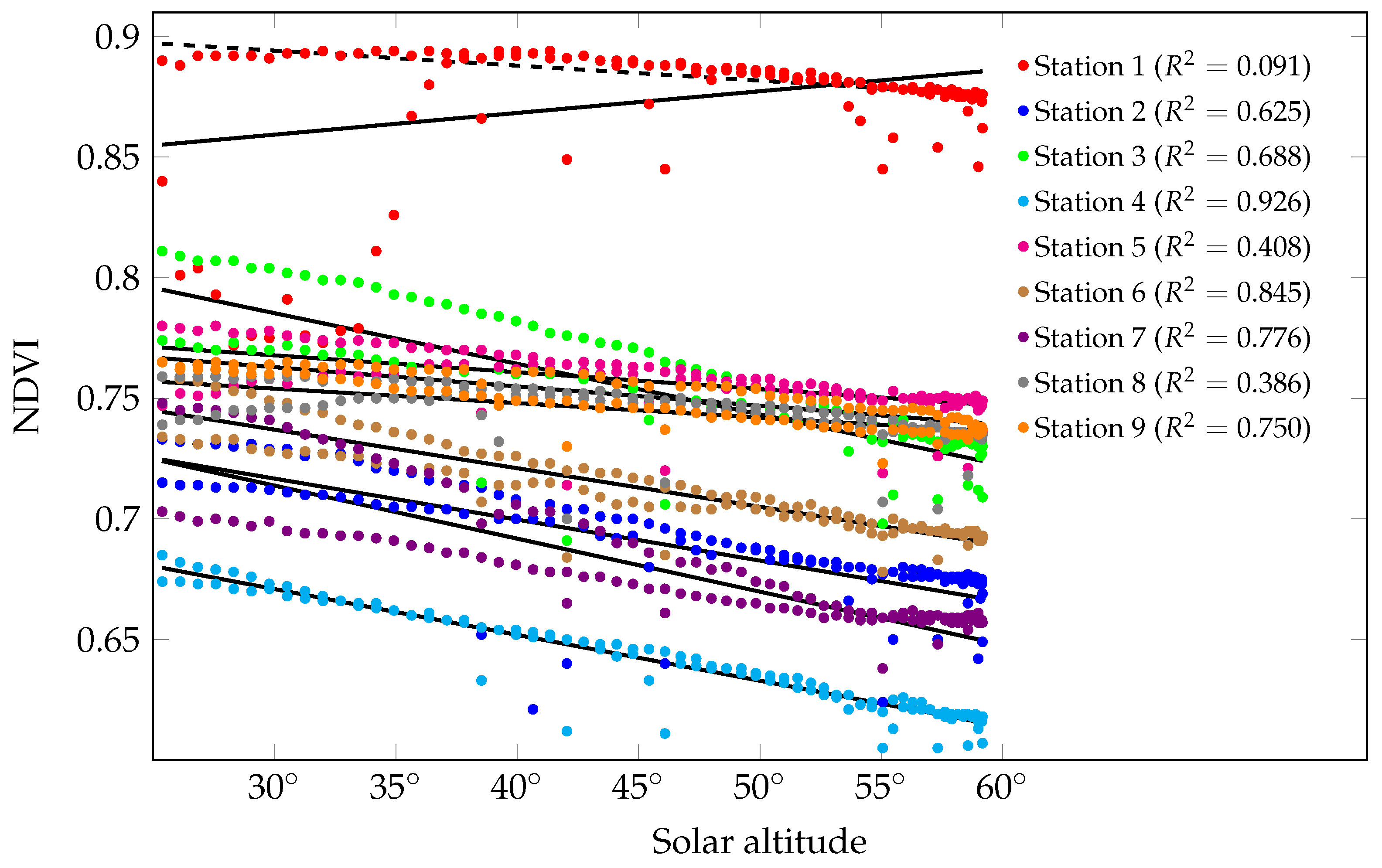
The reflectance spectra of the available S2 data were extracted for the close-range measurement stations. Based on these RS data, different spectral indices have been computed and compared with the computed data measured at close range. The computed spectral indices are listed in

Table 4. Overview of the calculated vegetation indices (modified according to Dahms et al. [64]).

Index	Equation	Remarks	Reference
NDVI	$\frac{NIR-R}{NIR+R}$	most commonly used vegetation index to describe the vegetation state	Rouse Jr et al. [23]
SAVI	$\frac{NIR-R}{NIR+R+L}(1+L)$	intended to minimize the effects of soil background on the vegetation signal	Huete [65]
RENDV	$\frac{R{E}_2-R{E}_1}{R{E}_2+R{E}_1}$	sensitive to vegetation in red edge	Gitelson and Merzlyak [66], Ahamed et al. [67]
RDVI	$\frac{NIR-R}{\sqrt{NIR+R}}$	sensitive to vegetation cover fraction variation	Roujean and Breon [68]
Symbol	Explanation
R	Red
$NIR$	Near Infrared
L	soil adjustment factor
$R{E}_1$	$705\mathrm{nm}$
$R{E}_2$	$740\mathrm{nm}$

.

3. Results

The pre-processing of the MSWN data consisted of the inter-calibration of the sensor pairs and the cross-calibration of S2A. In the case of the inter-calibration, all linear regressions of the close-range light sensors with hemispherical–conical sensor pairs resulted in adequate coefficients of determination ($R^2\ge 0.95$). Subsequently, the individual sensitivity ratios were applied to the data sets as a corrector.

Figure 6 illustrates the RSRs of S2A and the MWSN nadir-oriented sensor of Station 1 of the visible and NIR spectrum. Since the installed close-range sensors are manufactured from the same filter plate, the spectral differences between the specific channels are considered negligible. Therefore, the spectral characteristics of Station 1 are discussed in this paper as an example for all MWSN stations. These adjustment factors were applied to compare the S2A data with the MWSN data.

The multi-temporal behavior of the NDVI for all close-range measurements on 11 June 2016 is shown in Figure 7. Between 04:00 and 18:30 UTC, the measurements show a parabola curve between both maxima (in morning and evening) on different NDVI levels. The minimum during the day is approximately between 09:00 UTC and 12:30 UTC (see Figure 7).

Figure 8 describes the multi-temporal behavior on the MWSN records in more detail. Here, linear regressions of the measured NDVI and solar altitude are plotted for each station. The corresponding time series of solar altitudes were determined for each position using Astropy, version 5.0 [69], and considering the atmospheric refraction. Solar altitudes smaller than ${25}^{°}$ were not considered, minimizing effects such as the shading of the plots from shadows cast by the surrounding vegetation. Therefore, the selected data set corresponds to a time period of 5:55–16:20 UTC. In general, except for Station 1, there is a strong or moderate negative correlation between the solar altitude and the close-range measured NDVI. These correlations support the observed slight depression of the NDVI during the daytime (see Figure 7). Due to the local effects at Station 1, no correlation is discernible using simple linear regression. Applying the Theil–Sen estimator [70,71] to the data set of Station 1, a method of robustly fitting a line to sample points and that is insensitive to outliers, results in a similar fitting slope compared to the other stations.

Figure 9 graphically demonstrates the locality, spread, and skewness groups of all measured and cross-calibrated reflectances of all MWSN stations during the significant overfly period for sun-synchronous EO satellites (09:15–12:15 UTC). In addition, the instantaneous reflectance and the corresponding S2A reflectance are given for the respective locations of the MWSN. It should be noted that, depending on the spectral waveband, several sensor nodes can be located in the same pixel of the S2A measurement. This may also differ for different S2A overflights. This applies to the following cases for 11 June 2016: Stations 2 and 3 are in the same pixel for S2A Channels 5, 6, and 8a, whereas Stations 8 and 9 are in the same pixel for S2A Channel 5. Furthermore, linear regressions, with corresponding coefficients of determination ($R^2$) and p-values (p), were applied to correlate the instantaneous reflectance with the determined median of the MSWN reflectance time series (09:15–12:15 UTC). Only a weak correlation was found at 665 nm ($R^2=0.332$; $p=0.105$); a moderate correlation was found at 865 nm ($R^2=0.644$; $p=0.009$) and 705 nm ($R^2=0.689$; $p=0.006$). A strong correlation was determined at 740 nm ($R^2=0.823$; $p=0.001$).

To compare the ground-based monitored spectral characteristics of the MWSN transect in more detail, the VIs listed in Table 4 for the MWSN based on the measurement closest to the S2A acquisition ($\Delta t<150 \mathrm{s}$) were calculated as well as for S2A. Figure 10 shows the development of different VIs depending on the distance to the Peene River ditch. While Figure 9 is intended to illustrate potential dynamics for the EO overfly period, the main focus of Figure 10 is to compare the near-instantaneous data sets directly and illustrate more stationary influences during this period, such as the soil signal and vegetation cover fraction, respectively. Furthermore, linear regressions were also determined concerning the near-instantaneous indices of Figure 10. The NDVI ($R^2=0.541$; $p=0.024$) shows only a moderate correlation between the MWSN and S2A. Strong correlations occur for the SAVI ($R^2=0.719$; $p=0.004$), RENDVI ($R^2=0.789$; $p=0.001$), and RDVI ($R^2=0.721$; $p=0.004$).

In addition to the instantaneous information, box plots based on the calculated NDVI for solar altitudes ≥${25}^{°}$ are also shown (see Figure 11) for the MWSN compared to the NDVI of S2A to visualize potential fluctuations. This is a general approach for MWSN data to document short-term effects (e.g., wind-induced change in vegetation reflectance). However, conditions were stable during the observation period on the day of 11 June 2016, as can be seen in Figure 7. Furthermore, an important aspect for consideration is the effect of vegetation types and climates as well as potential variation in the NDVI of the effective full cover on a maximum value of the NDVI (NDVImax). For different EO satellite missions, a compilation was given by Shah et al. [72]. This compilation illustrates the range of NDVImax values from 0.65 for Senegal, West Africa [73] to 0.7 in the northern boreal forests of Canada [74] and up to 0.996 for the Iberian Peninsula [75]. For the DEMMIN area, an NDVImax value of 0.95 was measured for Landsat 7 ETM+ [31]. Figure 11 shows the individual ground-based NDVI variations in comparison to a selection of NDVImax measured worldwide.

4. Discussion

The development of the NDVI (Figure 7) at the measurement stations depends on the monitored vegetation and site factors and stressors (e.g., water supply, soil density, nutrient supply) of the selected transect along the elevation profile in the field. Comparative observation of the fundamental environmental and pedological situation (Figure 3 and Table 3) of the MWSN stations allows an initial assessment of the influence regarding the close-range measurements. The spectral measurements at Station 1 show a signature of dense, vital vegetation. This is reflected in high (>0.8) vegetation on Stations 2 and 3, where loose vegetation in the direct headland of the field (and, therefore, heavily compressed) was characterized by natural vegetation types. The following six stations were located in the winter canola field. The significantly lower NDVI for these stations indicates non-optimal growth conditions in these areas and the simple absence of vegetation due to the driveway.

The NDVI curve progression at all stations (Figure 7) and corresponding linear regressions (Figure 8) demonstrate the influence of the solar zenith angle on the NDVI measurements. In general, the vegetation index decreased with increasing solar altitude (Figure 8). This is consistent with the results of Ishihara et al. [76] for different vegetation types with clear sky conditions for solar altitudes higher than ${30}^{°}$. Therefore, seasonal differences due to other typical solar courses cannot be excluded. Under cloudy sky conditions, Ishihara et al. [76] did not find a clear linear relationship. Since canopy reflectance is affected by the view and illumination geometry, the canopy structure, optical properties of the vegetation, and the soil conditions [76,77,78,79], a correction of vegetation indices derived, e.g., by a radiative transfer model for respective land cover classes, is a key procedure. Accordingly, the response of the canopy reflectance to the solar zenith angle is determined by the interactive effects of the canopy structure (the LAI and leaf angle distribution) or by the BRDF, respectively, of the canopy and soil surface [76]. Usually, sun-synchronous satellite-based remote sensing missions collect data between 9:15–12:15 UTC in Central Europe. This corresponds with the time slot of diurnal minimum between the morning and evening maximum of the ground-based measured NDVI, exemplarily shown for S2 in Figure 7. This effect indicates that, depending on the overflight time of an EO mission, the reflectance or vegetation indices determined in a corresponding manner can vary enormously without a corresponding correction.

Figure 7 also illustrates the significantly different NDVI signal behavior of the stations during sunrise and sunset. This can be attributed to topological conditions such as the strong slope in the trench area (see Figure 3). Therefore, depending on the location in the transect, depressions (e.g., Station 1) or time-shifted progressions may occur during this period. However, this cannot be clarified using the available data.

Figure 9 shows that, overall, the spectral components of the observed frequency bands correlate well with the reflectances of S2A in the red edge and correlate less in the red or the NIR range. However, depending on the respective MWSN station, the red, red edge, and NIR channels of the close-range sensors show slightly higher or lower reflectances in some cases, as calculated for S2A. The cause of this effect could be the varying portion of the soil signal during the measurement since small-scale heterogeneity in the FOV of the sensor network can have a significant influence. A typical bare soil or vegetation–soil mixture usually has a significantly higher reflectance in the red waveband and lower reflectances in the red edge and NIR compared to dense green vegetation [80,81,82]. This also correlates with the observations of the identified VIs (see Figure 10). There are more significant deviations in the NDVI ($R^2=0.541$; $p=0.024$) between the MWSN and S2A than in the case with the SAVI ($R^2=0.719$; $p=0.004$), which is estimated from the same input data as the NDVI but was developed to minimize such influences. However, besides the heterogeneity in the FOV of the close-range sensors, some deviation could be attributed to sub-pixel heterogeneity. As mentioned in the results, Stations 8 and 9 are located in the same pixel during the corresponding S2A overflight for Channel 5 (reflectance at 705 nm). Here (Figure 9), the determined reflectance of S2A corresponds approximately to the mean of the two time series of the close-range sensors and indicates the integrative signal but needs to be further investigated for validation.

Another distinctive feature in Figure 9 is that the signal scatter significantly varies depending on the stations’ location in the transect. This could be caused by the influence of vegetation height, or the LAI, on the close-range measurements. The optical thickness of a canopy and the illuminated components of vegetation or background highly influence the diurnal variations in reflectance [76,83]. In most crop canopies, the canopy reflectance is determined mainly by the soil reflectance in small LAI conditions (≈1) and by the vegetation reflectance in large LAI conditions (≈4) [76]. The reflectance scatter is lowest in the headland and increases over the natural meadow to the canola, where the most substantial variations occur. Here, the shading of the lower parts of the vegetation stand is a possible driving factor.

However, Station 9 also shows a relatively slight variation in the scatter. This implies a more exposed FOV, which should contain more soil signal. Comparing the close-range channels with the S2A measurements, as well as the field observations, confirms this (see Figure 4c). Station 8 shows a lower reflectance in the red waveband and correspondingly lower reflectances for the red edge and NIR than S2A, as expected from a higher share of soil signal. In addition, the slight variations at Station 1 could be influenced by the relatively homogeneous FOV of the natural meadow. The reason for the large scatter at Station 8 at 740 nm is slightly unclear. It is not due to a typical outlier since several nonconsecutive values define the lower whisker of the boxplot. In contrast, the first and third quartiles show plausible data. Therefore, this should nevertheless be classified as an outlier.

When increasing distances from the water ditch of the Peene River, the MWSN stations, as well as S2A, show lower values for all of the calculated VIs of more sparse vegetation (Station 2–4; see Figure 10). In addition, the strongest variances between both data sets also occur in this transect section, as Figure 11 shows that spontaneous or highly dynamic processes do not cause these deviations since the measurement times are shifted by up to 150 s. The statistical evaluation of the measured close-range reflectances (see Figure 9) during the significant overfly period for sun-synchronous opto-electronical satellites shows that these deviations must be caused systematically. Some of these effects may be caused by the heterogeneity of the canola stand at the subpixel level. However, this does not explain the offset of all of the VIs of Station 7, which could be due to a misaligned sensor head.

As highlighted by Figure 7, the view and illumination geometry also significantly influence all of the VIs. This becomes apparent when considering the effect of vegetation types and climates as well as the potential variation in NDVI caused by effective full cover on the NDVI’s maximum value (see Figure 11). Station 1, which can be regarded as effective full cover, shows that, e.g., the effect of vegetation type is very much dominated by the influence of the respective BRDF. In general, diurnal responses are affected by the differences in canopy structure and the growth pattern for each vegetation type [76]. Therefore, it is necessary to correct this influence in the close-range measurements of the MWSN data and in the RS data, such as the S2 scenes, to improve the inter-comparability of both data sources. These corrective steps can minimize the uncertainties between close-range measurements and remote sensing [40,84].

5. Conclusions

Because neither RS nor ground-based close-range measurements can usually cover all information requirements exclusively to describe, e.g., an ecosystem function, an optimized combination of both techniques that specifically targets the problem is required. Furthermore, the necessity for an integrated measurement system is evident. It would feature a favorable, synergistically effective function sharing of ground-based measurements and RS to leverage the benefits of each measurement system and minimize their drawbacks. Therefore, the presented study represents key challenges of the interplay of in situ and RS data in several respects: the uncertain spatiotemporal availability of remote sensing products, the ad hoc validation of multispectral data in an agricultural context, and the continuous collection of similar sensed data on the ground and in space, which networks such as DEMMIN cannot realize using their automated monitoring program.

Especially in the context of studies of the net ecosystem exchange (NEE) of, e.g., carbon dioxide, accurate knowledge of the diurnal cycle of vegetation is an essential prerequisite for understanding the system [85]. In this context, daily variations in the NEE for mountain grasslands, for example, have been primarily related to PPFD and soil and air temperature [85], while seasonal variations have been linked to changes in the LAI [85,86]. In both cases, the NDVI can be evaluated as an indicator to track vegetation behavior [85,86,87]. Systems that provide accurate knowledge of the spatiotemporal diurnal variation in NDVI values are particularly geostationary satellites that allow monitoring of daily ecosystem dynamics [86,87]. Ground-based close-range observations can provide detailed and accurate information on the dynamic change in structure or function of vegetation based on high temporal resolution data and can be used for the absolute calibration of satellite or airborne images [76]. However, these data are affected by the solar altitude and the current light conditions at the time of data recording. In addition, the continuous collection of such long-term data sets can be challenging because access, e.g., to arable land, is limited in time. A suitable measurement program for recording such ecosystem exchange processes would therefore result in a methodology such as this:

• Multi-temporal measurements with the same satellite from different orbits (positions);
• Measurements with geostationary satellites at different times of the day;
• Measurements with gonioreflectometer for measuring BRDF;
• Measurements with UAVs in a goniometer-simulating configuration;
• Continuous measurements with ground-based close-range sensor systems.

However, for terrestrial ecosystems, or systems of potentially unlimited complexity and heterogeneity, the amount and quality of data limit the amount of extractable knowledge [88]. Rose et al. [89] suggest how human activities are altering the scales of ecological processes, resulting in interactions at novel space–time scale combinations that are diverse and predictable. In addition, global change affects the Earth and the environment on many temporal and spatial scales. Currently, only limited knowledge is available on the importance of distinct dynamic events for the long-term development of environmental systems [90]. To adequately describe these relations and processes, harmonized high-quality data on the continental scale are required and tools need to be developed to meet the new challenges of technological advances and scientific progress: space-borne and ground-based [5]. Therefore, e.g., one of Europe’s key challenges is the transformation of existing in situ research sites into harmonized, high-performance, complementary, and interoperable socio-ecosystem research infrastructures [5] to provide the European counterpart to other continental-scale ecological research infrastructures such as the US National Ecological Observatory Network [91] or the Australian Terrestrial Ecosystem Research Network [92]. Existing harmonization initiatives such as the Long-term Ecological Research Network (LTER)’s framework for standard observations provide a harmonized guiding principle for designing a pan-European infrastructure and for future infrastructural enhancements of LTER-Europe sites [5]. An MWSN can support stationary networks and RS products as an ad hoc complement to routine measurement programs. The possibility of adapting the spectral characteristics of the networks to the corresponding missions represents a cost-effective alternative that can especially play a decisive role in future data analysis and should be further investigated for other EO satellite missions. This results in a spatial and temporal compression of the measurement programs or an extension of the parameters for the processes to be observed and can bridge existing spatiotemporal gaps, allowing European EO satellite missions, such as S2, to reach their full potential, given the availability of adequate ground truth data.

References

1. Gascon, F.; Cadau, E.; Colin, O.; Hoersch, B.; Isola, C.; Fernández, B.L.; Martimort, P. Copernicus Sentinel-2 mission: Products, algorithms and Cal/Val. In Proceedings of the Earth Observing Systems XIX, SPIE, San Diego, CA, USA, 17–21 August 2014; Volume 9218, pp. 455–463. [Google Scholar]
2. Drusch, M.; Del Bello, U.; Carlier, S.; Colin, O.; Fernandez, V.; Gascon, F.; Hoersch, B.; Isola, C.; Laberinti, P.; Martimort, P.; et al. Sentinel-2: ESA’s optical high-resolution mission for GMES operational services. Remote Sens. Environ. 2012, 120, 25–36. [Google Scholar] [CrossRef]
3. Irons, J.R.; Dwyer, J.L.; Barsi, J.A. The next Landsat satellite: The Landsat data continuity mission. Remote Sens. Environ. 2012, 122, 11–21. [Google Scholar] [CrossRef]
4. Zacharias, S.; Bogena, H.; Samaniego, L.; Mauder, M.; Fuß, R.; Pütz, T.; Frenzel, M.; Schwank, M.; Baessler, C.; Butterbach-Bahl, K.; et al. A network of terrestrial environmental observatories in Germany. Vadose Zone J. 2011, 10, 955–973. [Google Scholar] [CrossRef]
5. Mollenhauer, H.; Kasner, M.; Haase, P.; Peterseil, J.; Wohner, C.; Frenzel, M.; Mirtl, M.; Schima, R.; Bumberger, J.; Zacharias, S. Long-term environmental monitoring infrastructures in Europe: Observations, measurements, scales, and socio-ecological representativeness. Sci. Total. Environ. 2018, 624, 968–978. [Google Scholar] [CrossRef] [PubMed]
6. Bogena, H.; Kunkel, R.; Puetz, T.; Vereecken, H.; Krueger, E.; Zacharias, S.; Dietrich, P.; Wollschlaeger, U.; Kunstmann, H.; Papen, H.; et al. Tereno-long-term monitoring network for terrestrial environmental research. Hydrol. Wasserbewirtsch. 2012, 56, 138–143. [Google Scholar]
7. Gaillardet, J.; Braud, I.; Hankard, F.; Anquetin, S.; Bour, O.; Dorfliger, N.; De Dreuzy, J.R.; Galle, S.; Galy, C.; Gogo, S.; et al. OZCAR: The French network of critical zone observatories. Vadose Zone J. 2018, 17, 1–24. [Google Scholar] [CrossRef]
8. Lausch, A.; Erasmi, S.; King, D.J.; Magdon, P.; Heurich, M. Understanding forest health with remote sensing-part I—A review of spectral traits, processes and remote-sensing characteristics. Remote Sens. 2016, 8, 1029. [Google Scholar] [CrossRef]
9. Ustin, S.L.; Gamon, J.A. Remote sensing of plant functional types. New Phytol. 2010, 186, 795–816. [Google Scholar] [CrossRef]
10. Lausch, A.; Borg, E.; Bumberger, J.; Dietrich, P.; Heurich, M.; Huth, A.; Jung, A.; Klenke, R.; Knapp, S.; Mollenhauer, H.; et al. Understanding Forest Health with Remote Sensing, Part III: Requirements for a Scalable Multi-Source Forest Health Monitoring Network Based on Data Science Approaches. Remote Sens. 2018, 10, 1120. [Google Scholar] [CrossRef]
11. Taramelli, A.; Tornato, A.; Magliozzi, M.L.; Mariani, S.; Valentini, E.; Zavagli, M.; Costantini, M.; Nieke, J.; Adams, J.; Rast, M. An Interaction Methodology to Collect and Assess User-Driven Requirements to Define Potential Opportunities of Future Hyperspectral Imaging Sentinel Mission. Remote Sens. 2020, 12, 1286. [Google Scholar] [CrossRef]
12. Asadzadeh, S.; de Souza Filho, C.R. Investigating the capability of WorldView-3 superspectral data for direct hydrocarbon detection. Remote Sens. Environ. 2016, 173, 162–173. [Google Scholar] [CrossRef]
13. Hase, N.; Doktor, D.; Rebmann, C.; Dechant, B.; Mollenhauer, H.; Cuntz, M. Identifying the main drivers of the seasonal decline of near-infrared reflectance of a temperate deciduous forest. Agric. For. Meteorol. 2022, 313, 108746. [Google Scholar] [CrossRef]
14. Schrön, M.; Zacharias, S.; Womack, G.; Köhli, M.; Desilets, D.; Oswald, S.E.; Bumberger, J.; Mollenhauer, H.; Kögler, S.; Remmler, P.; et al. Intercomparison of cosmic-ray neutron sensors and water balance monitoring in an urban environment. Geosci. Instrum. Methods Data Syst. 2018, 7, 83–99. [Google Scholar] [CrossRef]
15. Fersch, B.; Francke, T.; Heistermann, M.; Schrön, M.; Döpper, V.; Jakobi, J.; Baroni, G.; Blume, T.; Bogena, H.; Budach, C.; et al. A dense network of cosmic-ray neutron sensors for soil moisture observation in a highly instrumented pre-Alpine headwater catchment in Germany. Earth Syst. Sci. Data 2020, 12, 2289–2309. [Google Scholar] [CrossRef]
16. Van den Bossche, J.; Peters, J.; Verwaeren, J.; Botteldooren, D.; Theunis, J.; De Baets, B. Mobile monitoring for mapping spatial variation in urban air quality: Development and validation of a methodology based on an extensive dataset. Atmos. Environ. 2015, 105, 148–161. [Google Scholar] [CrossRef]
17. Tessum, M.W.; Larson, T.; Gould, T.R.; Simpson, C.D.; Yost, M.G.; Vedal, S. Mobile and fixed-site measurements to identify spatial distributions of traffic-related pollution sources in Los Angeles. Environ. Sci. Technol. 2018, 52, 2844–2853. [Google Scholar] [CrossRef]
18. Holmgren, J.; Fredriksson, H.; Dahl, M. On the use of active mobile and stationary devices for detailed traffic data collection: A simulation-based evaluation. Int. J. Traffic Transp. Manag. 2021, 3, 1–9. [Google Scholar]
19. Koch, K.; Schade, G.W.; Filippi, A.M.; Goessler, G.; Güneralp, B. Low-Key Stationary and Mobile Tools for Probing the Atmospheric UHI Effect. In Spatial Variability in Environmental Science-Patterns, Processes, and Analyses; IntechOpen: London, UK, 2019. [Google Scholar]
20. Viana, M.; Rivas, I.; Reche, C.; Fonseca, A.S.; Pérez, N.; Querol, X.; Alastuey, A.; Álvarez-Pedrerol, M.; Sunyer, J. Field comparison of portable and stationary instruments for outdoor urban air exposure assessments. Atmos. Environ. 2015, 123, 220–228. [Google Scholar] [CrossRef]
21. Borg, E. CAL/VAL Site DEMMIN for Remote Sensing. Network of European Regions Using Space Technology; NEREUS Earth Observation/GMES Working Group: Brussels, Belgium, 2010; pp. 13–14. [Google Scholar]
22. Jordan, C.F. Derivation of leaf-area index from quality of light on the forest floor. Ecology 1969, 50, 663–666. [Google Scholar] [CrossRef]
23. Rouse, J., Jr.; Haas, R.; Schell, J.; Deering, D. Monitoring vegetation systems in the Great Plains with ERTS. In Third Earth Resources Technology Satellite-1 Symposium: Volume 1; Freden, S.C., Mercanti, E.P., Becker, M.A., Eds.; Technical Presentations, Section B; NASA Special Publ. Technical Report, NASA-SP-351-VOL-1-SECT-B, A 20; NASA: Washington, DC, USA, 1974; pp. 309–317. [Google Scholar]
24. Monsi, M. Über den Lichtfaktor in den Pflanzengesellschaften und seine Bedeutung fur die Stoffproduktion. Jap. J. Bot. 1953, 14, 22–52. [Google Scholar]
25. Yao, Y.; Liu, Q.; Liu, Q.; Li, X. LAI retrieval and uncertainty evaluations for typical row-planted crops at different growth stages. Remote Sens. Environ. 2008, 112, 94–106. [Google Scholar] [CrossRef]
26. Zheng, G.; Moskal, L.M. Retrieving leaf area index (LAI) using remote sensing: Theories, methods and sensors. Sensors 2009, 9, 2719–2745. [Google Scholar] [CrossRef] [PubMed]
27. Viña, A.; Gitelson, A.A.; Nguy-Robertson, A.L.; Peng, Y. Comparison of different vegetation indices for the remote assessment of green leaf area index of crops. Remote Sens. Environ. 2011, 115, 3468–3478. [Google Scholar] [CrossRef]
28. de Jong, S.M.; Jetten, V. Estimating spatial patterns of rainfall interception from remotely sensed vegetation indices and spectral mixture analysis. Int. J. Geogr. Inf. Sci. 2007, 21, 529–545. [Google Scholar] [CrossRef]
29. Hope, A.; Engstrom, R.; Stow, D. Relationship between AVHRR surface temperature and NDVI in Arctic tundra ecosystems. Int. J. Remote Sens. 2005, 26, 1771–1776. [Google Scholar] [CrossRef]
30. Sun, D.; Kafatos, M. Note on the NDVI-LST Relationship and the Use of Temperature-Related Drought Indices Over North America. Geophys. Res. Lett. 2007, 34, L24406. [Google Scholar] [CrossRef]
31. Wloczyk, C.; Borg, E.; Richter, R.; Miegel, K. Estimation of instantaneous air temperature above vegetation and soil surfaces from Landsat 7 ETM+ data in northern Germany. Int. J. Remote Sens. 2011, 32, 9119–9136. [Google Scholar] [CrossRef]
32. Gamon, J.A.; Field, C.B.; Goulden, M.L.; Griffin, K.L.; Hartley, A.E.; Joel, G.; Peñuelas, J.; Valentini, R. Relationships between NDVI, canopy structure, and photosynthesis in three Californian vegetation types. Ecol. Appl. 1995, 5, 28–41. [Google Scholar] [CrossRef]
33. Myneni, R.; Williams, D. On the relationship between FAPAR and NDVI. Remote Sens. Environ. 1994, 49, 200–211. [Google Scholar] [CrossRef]
34. Huang, J.; Wang, H.; Dai, Q.; Han, D. Analysis of NDVI data for crop identification and yield estimation. IEEE J. Sel. Top. Appl. Earth Obs. Remote Sens. 2014, 7, 4374–4384. [Google Scholar] [CrossRef]
35. Bolton, D.K.; Friedl, M.A. Forecasting crop yield using remotely sensed vegetation indices and crop phenology metrics. Agric. For. Meteorol. 2013, 173, 74–84. [Google Scholar] [CrossRef]
36. Mahlein, A.K.; Rumpf, T.; Welke, P.; Dehne, H.W.; Plümer, L.; Steiner, U.; Oerke, E.C. Development of spectral indices for detecting and identifying plant diseases. Remote Sens. Environ. 2013, 128, 21–30. [Google Scholar] [CrossRef]
37. Mulders, M.A. Remote Sensing in Soil Science; Elsevier: Amsterdam, The Netherlands, 1987. [Google Scholar]
38. Lausch, A.; Baade, J.; Bannehr, L.; Borg, E.; Bumberger, J.; Chabrilliat, S.; Dietrich, P.; Gerighausen, H.; Glässer, C.; Hacker, J.M.; et al. Linking remote sensing and geodiversity and their traits relevant to biodiversity—Part I: Soil characteristics. Remote Sens. 2019, 11, 2356. [Google Scholar] [CrossRef]
39. Vermote, E.; Vermeulen, A. Atmospheric correction algorithm: Spectral reflectances (MOD09). ATBD Version 1999, 4, 1–107. [Google Scholar]
40. Mannschatz, T.; Pflug, B.; Borg, E.; Feger, K.H.; Dietrich, P. Uncertainties of LAI estimation from satellite imaging due to atmospheric correction. Remote Sens. Environ. 2014, 153, 24–39. [Google Scholar] [CrossRef]
41. Gong, P.; Pu, R.; Biging, G.S.; Larrieu, M.R. Estimation of forest leaf area index using vegetation indices derived from Hyperion hyperspectral data. IEEE Trans. Geosci. Remote Sens. 2003, 41, 1355–1362. [Google Scholar] [CrossRef]
42. Reid, W.V.; Bréchignac, C.; Tseh Lee, Y. Earth System Research Priorities. Science 2009, 325, 245. [Google Scholar] [CrossRef]
43. Richter, D.D., Jr.; Mobley, M.L. Monitoring Earth’s critical zone. Science 2009, 326, 1067–1068. [Google Scholar] [CrossRef] [PubMed]
44. Teucher, M.; Thürkow, D.; Alb, P.; Conrad, C. Digital In Situ Data Collection in Earth Observation, Monitoring and Agriculture—Progress towards Digital Agriculture. Remote Sens. 2022, 14, 393. [Google Scholar] [CrossRef]
45. Gerighausen, H.; Borg, E.; Fichtelmann, B.; Günther, A.; Vajen, H.H.; Wloczyk, C.; Maass, H. Validation and calibration of remote sensing data products on test site DEMMIN. In Proceedings of the 43. Ziolkowski Conference, 43. Ziolkowski Conference, Kaluga, Russia, 16–18 September 2008. [Google Scholar]
46. Borg, E.; Schiller, C.; Daedelow, H.; Fichtelmann, B.; Jahncke, D.; Renke, F.; Tamm, H.P.; Asche, H. Automated generation of value-added products for the validation of remote sensing information based on in-situ data. In Proceedings of the International Conference on Computational Science and Its Applications, Guimarães, Portugal, 30 June–3 July 2014; pp. 393–407. [Google Scholar]
47. Götze, M.; Kattanek, W.; Peukert, R.; Chervakova, E.; Töpfer, H.; Dietrich, P.; Bumberger, J.; of Electrical, I.; Engineers, E. A flexible service and communication gateway for monitoring applications. In Proceedings of the 21st International Conference on Software, Telecommunications and Computer Networks (SoftCOM), Split-Primosten, Croatia, 18–20 September 2013; pp. 1–5. [Google Scholar]
48. Töpfer, H.; Chervakova, E.; Goetze, M.; Hutschenreuther, T.; Nikolić, B.; Dimitrijević, B. Application of wireless sensors within a traffic monitoring system. In Proceedings of the 2015 23rd Telecommunications Forum Telfor (TELFOR), Belgrade, Serbia, 24–26 November 2015; pp. 236–241. [Google Scholar]
49. Shelby, Z.; Bormann, C. 6LoWPAN: The Wireless Embedded Internet; John Wiley & Sons: Hoboken, NJ, USA, 2011. [Google Scholar]
50. Montenegro, G.; Kushalnagar, N.; Hui, J.; Culler, D. Transmission of IPv6 Packets over IEEE 802.15. 4 Networks. RFC Ser. 4944 2007. [Google Scholar] [CrossRef]
51. Mills, D. Simple network time protocol (SNTP) version 4 for IPv4, IPv6 and OSI. RFC Ser. 2030 1996. [Google Scholar] [CrossRef]
52. Agre, J.R.; Clare, L.P.; Pottie, G.J.; Romanov, N.P. Development platform for self-organizing wireless sensor networks. In Proceedings of the Unattended Ground Sensor Technologies and Applications, Orlando, FL, USA, 8–9 April 1999; Volume 3713, pp. 257–268. [Google Scholar]
53. Akitsu, T.; Nasahara, K.N.; Hirose, Y.; Ijima, O.; Kume, A. Quantum sensors for accurate and stable long-term photosynthetically active radiation observations. Agric. For. Meteorol. 2017, 237, 171–183. [Google Scholar] [CrossRef]
54. National Aeronautics and Space Administration. Sentinel-2A Launches—Our Compliments & Our Complements. Available online: https://landsat.gsfc.nasa.gov/article/sentinel-2a-launches-our-compliments-our-complements/ (accessed on 9 September 2023).
55. European Space Agency. SENTINEL-2 MISSION GUIDE. Available online: https://sentinels.copernicus.eu/web/sentinel/missions/sentinel-2 (accessed on 9 September 2023).
56. Malenovskỳ, Z.; Rott, H.; Cihlar, J.; Schaepman, M.E.; García-Santos, G.; Fernandes, R.; Berger, M. Sentinels for science: Potential of Sentinel-1,-2, and-3 missions for scientific observations of ocean, cryosphere, and land. Remote Sens. Environ. 2012, 120, 91–101. [Google Scholar] [CrossRef]
57. Slater, P.N.; Biggar, S.F.; Palmer, J.M.; Thome, K.J. Unified approach to absolute radiometric calibration in the solar-reflective range. Remote Sens. Environ. 2001, 77, 293–303. [Google Scholar] [CrossRef]
58. Chander, G.; Mishra, N.; Helder, D.L.; Aaron, D.B.; Angal, A.; Choi, T.; Xiong, X.; Doelling, D.R. Applications of spectral band adjustment factors (SBAF) for cross-calibration. IEEE Trans. Geosci. Remote Sens. 2012, 51, 1267–1281. [Google Scholar] [CrossRef]
59. Khakurel, P.; Leigh, L.; Kaewmanee, M.; Pinto, C.T. Extended Pseudo Invariant Site-Based Trend-to-Trend Cross-Calibration of Optical Satellite Sensors. Remote Sens. 2021, 13, 1545. [Google Scholar] [CrossRef]
60. Teillet, P.; Fedosejevs, G.; Thome, K.; Barker, J.L. Impacts of spectral band difference effects on radiometric cross-calibration between satellite sensors in the solar-reflective spectral domain. Remote Sens. Environ. 2007, 110, 393–409. [Google Scholar] [CrossRef]
61. Thuillier, G.; Hersé, M.; Labs, D.; Foujols, T.; Peetermans, W.; Gillotay, D.; Simon, P.C.; Mandel, H. The solar spectral irradiance from 200 to 2400 nm as measured by the SOLSPEC spectrometer from the ATLAS and EURECA missions. Sol. Phys. 2003, 214, 1–22. [Google Scholar] [CrossRef]
62. European Space Agency. Sentinel-2 Spectral Response Functions (S2-SRF), Technical Document S2-SRF_COPE-GSEG-EOPG-TN-15-0007_3.1. Available online: https://sentinels.copernicus.eu/web/sentinel/user-guides/sentinel-2-msi/document-library/-/asset_publisher/Wk0TKajiISaR/content/sentinel-2a-spectral-responses (accessed on 9 September 2023).
63. Jin, H.; Eklundh, L. In situ calibration of light sensors for long-term monitoring of vegetation. IEEE Trans. Geosci. Remote Sens. 2014, 53, 3405–3416. [Google Scholar] [CrossRef]
64. Dahms, T.; Seissiger, S.; Borg, E.; Vajen, H.; Fichtelmann, B.; Conrad, C. Important variables of a rapideye time series for modelling biophysical parameters of winter wheat. Photogramm.-Fernerkund.-Geoinf. 2016, 2016, 285–299. [Google Scholar] [CrossRef]
65. Huete, A. Huete, AR A soil-adjusted vegetation index (SAVI). Remote Sensing of Environment. Remote Sens. Environ. 1988, 25, 295–309. [Google Scholar] [CrossRef]
66. Gitelson, A.; Merzlyak, M.N. Quantitative estimation of chlorophyll-a using reflectance spectra: Experiments with autumn chestnut and maple leaves. J. Photochem. Photobiol. Biol. 1994, 22, 247–252. [Google Scholar] [CrossRef]
67. Ahamed, T.; Tian, L.; Zhang, Y.; Ting, K. A review of remote sensing methods for biomass feedstock production. Biomass Bioenergy 2011, 35, 2455–2469. [Google Scholar] [CrossRef]
68. Roujean, J.L.; Breon, F.M. Estimating PAR absorbed by vegetation from bidirectional reflectance measurements. Remote Sens. Environ. 1995, 51, 375–384. [Google Scholar] [CrossRef]
69. Astropy Collaboration; Price-Whelan, A.M.; Lim, P.L.; Earl, N.; Starkman, N.; Bradley, L.; Shupe, D.L.; Patil, A.A.; Corrales, L.; Brasseur, C.E.; et al. The Astropy Project: Sustaining and Growing a Community-oriented Open-source Project and the Latest Major Release (v5.0) of the Core Package. Astrophys. J. 2022, 935, 167. [Google Scholar] [CrossRef]
70. Theil, H. A rank-invariant method of linear and polynomial regression analysis. Indag. Math. 1950, 12, 173. [Google Scholar]
71. Sen, P.K. Estimates of the regression coefficient based on Kendall’s tau. J. Am. Stat. Assoc. 1968, 63, 1379–1389. [Google Scholar] [CrossRef]
72. Shah, D.; Pandya, M.; Trivedi, H.; Jani, A. Estimating minimum and maximum air temperature using MODIS data over Indo-Gangetic Plain. J. Earth Syst. Sci. 2013, 122, 1593–1605. [Google Scholar] [CrossRef]
73. Stisen, S.; Sandholt, I.; Nørgaard, A.; Fensholt, R.; Eklundh, L. Estimation of diurnal air temperature using MSG SEVIRI data in West Africa. Remote Sens. Environ. 2007, 110, 262–274. [Google Scholar] [CrossRef]
74. Czajkowski, K.P.; Mulhern, T.; Goward, S.N.; Cihlar, J.; Dubayah, R.O.; Prince, S.D. Biospheric environmental monitoring at BOREAS with AVHRR observations. J. Geophys. Res. Atmos. 1997, 102, 29651–29662. [Google Scholar] [CrossRef]
75. Nieto, H.; Sandholt, I.; Aguado, I.; Chuvieco, E.; Stisen, S. Air temperature estimation with MSG-SEVIRI data: Calibration and validation of the TVX algorithm for the Iberian Peninsula. Remote Sens. Environ. 2011, 115, 107–116. [Google Scholar] [CrossRef]
76. Ishihara, M.; Inoue, Y.; Ono, K.; Shimizu, M.; Matsuura, S. The Impact of Sunlight Conditions on the Consistency of Vegetation Indices in Croplands—Effective Usage of Vegetation Indices from Continuous Ground-Based Spectral Measurements. Remote Sens. 2015, 7, 14079–14098. [Google Scholar] [CrossRef]
77. Hatfield, J.; Gitelson, A.; Schepers, J.; Walthall, C. Application of spectral remote sensing for agronomic decisions. Agron. J. 2008, 100, S117–S131. [Google Scholar] [CrossRef]
78. Jacquemoud, S.; Verhoef, W.; Baret, F.; Bacour, C.; Zarco-Tejada, P.J.; Asner, G.P.; François, C.; Ustin, S.L. PROSPECT+ SAIL models: A review of use for vegetation characterization. Remote Sens. Environ. 2009, 113, S56–S66. [Google Scholar] [CrossRef]
79. Verhoef, W. Earth observation modeling based on layer scattering matrices. Remote Sens. Environ. 1985, 17, 165–178. [Google Scholar] [CrossRef]
80. Govender, M.; Chetty, K.; Bulcock, H. A review of hyperspectral remote sensing and its application in vegetation and water resource studies. Water Sa 2007, 33, 145–151. [Google Scholar] [CrossRef]
81. Baldridge, A.M.; Hook, S.J.; Grove, C.; Rivera, G. The ASTER spectral library version 2.0. Remote Sens. Environ. 2009, 113, 711–715. [Google Scholar] [CrossRef]
82. Li, Z.; Guo, X. A suitable vegetation index for quantifying temporal variation of leaf area index (LAI) in semiarid mixed grassland. Can. J. Remote Sens. 2010, 36, 709–721. [Google Scholar] [CrossRef]
83. Epiphanio, J.N.; Huete, A.R. Dependence of NDVI and SAVI on sun/sensor geometry and its effect on fAPAR relationships in Alfalfa. Remote Sens. Environ. 1995, 51, 351–360. [Google Scholar] [CrossRef]
84. Holzer-Popp, T.; Bittner, M.; Borg, E.; Dech, S.; Erbertseder, T.; Fichtelmann, B.; Schroedter, M. Process for Correcting Atmospheric Influences in Multispectral Optical Remote Sensing. U.S. Patent No. 6,484,099 B1, 19 November 2002. [Google Scholar]
85. Schmitt, M.; Bahn, M.; Wohlfahrt, G.; Tappeiner, U.; Cernusca, A. Land use affects the net ecosystem CO2 exchange and its components in mountain grasslands. Biogeosciences 2010, 7, 2297–2309. [Google Scholar] [CrossRef]
86. Kim, S.i.; Ahn, D.S.; Han, K.S.; Yeom, J.M. Improved Vegetation Profiles with GOCI Imagery Using Optimized BRDF Composite. J. Sens. 2016, 2016, 7165326. [Google Scholar] [CrossRef]
87. Uudus, B.; Park, K.A.; Kim, K.R.; Kim, J.; Ryu, J.H. Diurnal variation of NDVI from an unprecedented high-resolution geostationary ocean colour satellite. Remote Sens. Lett. 2013, 4, 639–647. [Google Scholar] [CrossRef]
88. Thierfelder, T.K.; Grayson, R.B.; von Rosen, D.; Western, A.W. Inferring the location of catchment characteristic soil moisture monitoring sites. Covariance structures in the temporal domain. J. Hydrol. 2003, 280, 13–32. [Google Scholar] [CrossRef]
89. Rose, K.C.; Graves, R.A.; Hansen, W.D.; Harvey, B.J.; Qiu, J.; Wood, S.A.; Ziter, C.; Turner, M.G. Historical foundations and future directions in macrosystems ecology. Ecol. Lett. 2017, 20, 147–157. [Google Scholar] [CrossRef]
90. Weber, U.; Attinger, S.; Baschek, B.; Boike, J.; Borchardt, D.; Brix, H.; Brüggemann, N.; Bussmann, I.; Dietrich, P.; Fischer, P.; et al. MOSES: A novel observation system to monitor dynamic events across Earth compartments. Bull. Am. Meteorol. Soc. 2021, 103, 1–23. [Google Scholar] [CrossRef]
91. Schimel, D.; Hargrove, W.; Hoffman, F.; MacMahon, J. NEON: A hierarchically designed national ecological network. Front. Ecol. Environ. 2007, 5, 59. [Google Scholar] [CrossRef]
92. Karan, M.; Liddell, M.; Prober, S.M.; Arndt, S.; Beringer, J.; Boer, M.; Cleverly, J.; Eamus, D.; Grace, P.; Van Gorsel, E.; et al. The Australian SuperSite Network: A continental, long-term terrestrial ecosystem observatory. Sci. Total Environ. 2016, 568, 1263–1274. [Google Scholar] [CrossRef]
Figure 1. Schematic diagram of the combination of different measurement systems as complementary tools to capture environmental properties (modified according to Borg [21]).
Remotesensing 15 04663 g001
Figure 2. Left: DEMMIN in Mecklenburg-Western Pomerania (red rectangle). Right: Agricultural fields are marked in yellow, and an enlarged image by S2A of the NDVI (11 June 2016) with pins (1–9) indicating the location of the MWSN nodes (modified according to [46]).
Remotesensing 15 04663 g002
Figure 3. The succession of nine soil profiles along the MWSN measurement transect. The soils indicate intense soil erosion at the hilltop and thick colluvial covers at the lower slope.
Remotesensing 15 04663 g003
Figure 4. The photographs show the vegetation cover on 2016/05/31. The plant cover at Position 1 was a natural meadow (a); at Position 3, a relatively naturally developed meadow in the range of the headland and the drive onto the field (b); and the canola cover at Position 9 (c). The scheme (d) illustrates an MWSN node measuring analogous to the spectral wavebands to S2.
Remotesensing 15 04663 g004
Figure 5. Schematic configuration of sensor pair calibration for a hemispherical–conical sensor pair (modified according to Jin and Eklundh [63]). The downward-facing conical FOV sensor (Sensor 2) and the white reference panel are considered a sensor system measuring an irradiance quantity that is assumed to be equal to the irradiance measured by the hemispherical view sensor (Sensor 1).
Remotesensing 15 04663 g005
Figure 6. Response functions of the analyzed S2A channels and the corresponding close-range sensor channels.
Remotesensing 15 04663 g006
Figure 7. Multi-temporal behavior of winter canola (NDVI) using ground truth data on 11 June 2016 (04:00–18:30 UTC) at different measurement stations.
Remotesensing 15 04663 g007
Figure 8. Comparison of the NDVI and solar altitude for each individual MWSN station for solar altitudes 25 ° on 2016/06/11. Solid lines indicate simple linear regression with the corresponding coefficient of determination ( R 2 ). The dashed line indicates the linear fit for Station 1 using the Theil–Sen estimator.
Remotesensing 15 04663 g008
Figure 9. Comparison of the locality, spread, and skewness groups of close-range reflectance for each individual MWSN station (blue boxplots) during the significant overfly period for sun-synchronous EO satellites (11 June 2016; 09:15–12:15 UTC) and the respective S2A band pixel measurements (red dots, 11 June 2016; 10:20 UTC) with increasing distance from the Peene River ditch.
Remotesensing 15 04663 g009aRemotesensing 15 04663 g009b
Figure 10. Comparison of the calculated close-range light sensor VIs closest to the S2A overflight ( Δ t < 150 s) vs. the S2A VIs (11 June 2016; 10:20 UTC) with increasing distance from the Peene River ditch.
Remotesensing 15 04663 g010
Figure 11. Plot-scale measured NDVI (blue boxplots) for each MWSN station during the day of 11 June 2016 for solar altitudes 25 ° (05:55–16:20 UTC) compared to a selection of worldwide estimated NDVImax [31,73,74] (colored lines) and the S2A data acquisition on 11 June 2016 at 10:20 UTC (red dots).
Remotesensing 15 04663 g011