the Creative Commons Attribution 4.0 License.
the Creative Commons Attribution 4.0 License.
 | 17 Aug 2023
Assessing environmental change associated with early Eocene hyperthermals in the Atlantic Coastal Plain, USA
William Rush
Jean Self-Trail
Yang Zhang
Appy Sluijs
Henk Brinkhuis
James Zachos
James G. Ogg
Marci Robinson
Eocene transient global warming events (hyperthermals) can provide insight into a future warmer world. While much research has focused on the Paleocene–Eocene Thermal Maximum (PETM), hyperthermals of a smaller magnitude can be used to characterize climatic responses over different magnitudes of forcing. This study identifies two events, namely the Eocene Thermal Maximum 2 (ETM2 and H2), in shallow marine sediments of the Eocene-aged Salisbury Embayment of Maryland, based on magnetostratigraphy, calcareous nannofossil, and dinocyst biostratigraphy, as well as the recognition of negative stable carbon isotope excursions (CIEs) in biogenic calcite. We assess local environmental change in the Salisbury Embayment, utilizing clay mineralogy, marine palynology, δ18O of biogenic calcite, and biomarker paleothermometry (TEX86). Paleotemperature proxies show broad agreement between surface water and bottom water temperature changes. However, the timing of the warming does not correspond to the CIE of the ETM2 as expected from other records, and the highest values are observed during H2, suggesting factors in addition to pCO2 forcing have influenced temperature changes in the region. The ETM2 interval exhibits a shift in clay mineralogy from smectite-dominated facies to illite-rich facies, suggesting hydroclimatic changes but with a rather dampened weathering response relative to that of the PETM in the same region. Organic walled dinoflagellate cyst assemblages show large fluctuations throughout the studied section, none of which seem systematically related to CIE warming. These observations are contrary to the typical tight correspondence between climate change and assemblages across the PETM, regionally and globally, and ETM2 in the Arctic Ocean. The data do indicate very warm and (seasonally) stratified conditions, likely salinity-driven, across H2. The absence of evidence for strong perturbations in local hydrology and nutrient supply during ETM2 and H2, compared to the PETM, is consistent with the less extreme forcing and the warmer pre-event baseline, as well as the non-linear response in hydroclimates to greenhouse forcing.
- Article
(3998 KB) - Full-text XML
- BibTeX
- EndNote


The early Eocene is punctuated by a series of transient phases of carbon input and global warming, which are termed hyperthermals (e.g., Thomas and Zachos, 2000; Cramer et al., 2003; Littler et al., 2014). The well-studied Paleocene–Eocene Thermal Maximum (PETM) may represent the closest approximation to modern-day warming in the geologic record (Zachos et al., 2008). However, debate exists as to the origins of this event with respect to the primary source of carbon (Zeebe and Lourens, 2019; Zachos et al., 2010; Reynolds et al., 2017; Dickens et al., 1997; Frieling et al., 2019; Gutjahr et al., 2017). The mass of C released and rise in pCO2 are constrained by records of seafloor carbonate dissolution and surface ocean pH (Zachos et al., 2005; Penman et al., 2014; Gutjahr et al., 2017). Along continental margins, for example, in the Salisbury Embayment located within the mid-Atlantic Coastal Plain of the United States, the PETM is marked by sedimentological and biotic evidence of strong hydrological perturbations (Kopp et al., 2009; Sluijs and Brinkhuis, 2009; Stassen et al., 2012b; Self-Trail et al., 2012, 2017b; Rush et al., 2021). The Eocene Thermal Maximum 2 (ETM2) occurred approximately ∼ 2 Myr after the PETM and is characterized by warming and carbon release of approximately one-third that of the PETM (Lourens et al., 2005; Sluijs et al., 2009; Stap et al., 2010; Dunkley Jones et al., 2013; Gutjahr et al., 2017; Harper et al., 2020). ETM2 can provide insight into the climatic impacts of a smaller carbon forcing (pCO2) when compared to the PETM from geographically similar sites and hence provide insight into sensitivity to greenhouse forcing.
Intensification of the hydrologic cycle is a critical feature of the climatic response to greenhouse forcing (e.g., Carmichael et al., 2017). Evidence for a pronounced mode shift during the PETM includes enhanced sediment fluxes in sections from the mid-Atlantic margin, which suggest an increased frequency of precipitation extremes leading to high-energy fluvial activity and the associated abundances of low-salinity-tolerant biota (John et al., 2008; Self-Trail et al., 2017b; Stassen et al., 2012b; Rush et al., 2021; Sluijs and Brinkhuis, 2009). Similar signals have been found in many regions across various hyperthermals, including the Pyrenees, the margins of the Tethys, Aotearoa / New Zealand, the North Sea basin, and the Arctic (Schmitz and Pujalte, 2007; Jiang et al., 2021; Slotnick et al., 2012; Sluijs et al., 2014, 2007; Jin et al., 2022; Harding et al., 2011). These changes in extreme precipitation patterns are consistent with projections for future change (Pfahl et al., 2017; Swain et al., 2018). Studying the impacts of hydroclimatic changes in response to differing degrees of carbon forcings can inform as to the linearity of these responses, called “tipping point” thresholds, and the background variability in the hydrosphere.
Given the extensive evidence of a mode shift in coastal mid-Atlantic hydroclimate during the PETM, we initiated a regional search for ETM2. We here identify ETM2 and H2 (∼ 54 Ma) in the Knapps Narrows core based on biostratigraphic, paleomagnetic, and chemostratigraphic data. We present proxy records of the regional climatic response, including foraminiferal δ18O- and TEX86-based temperature reconstructions, clay mineralogy, and organic walled dinoflagellate cyst (dinocyst) assemblages and compare the results to published records of the PETM from this region.
2.1 Material
The Knapps Narrows core was drilled at 38.72129∘ N, 76.33162∘ W on the eastern shore of Maryland, in close proximity to drill sites which have been extensively studied for the PETM, South Dover Bridge, and Howards Tract (Fig. 1). The cored target interval lies between 84–102 m in the Nanjemoy Formation, an Eocene glauconitic sand in the upper Pamunkey group deposited in a shallow marine environment (Darton, 1951; Self-Trail et al., 2017b). From the bottom of the section to 88.4 m, the lithology is dominated by very coarse- to fine-grained, poorly sorted, angular to subrounded sand, comprised of ∼ 50 % glauconite, ∼ 30 % quartz, and < 5 % muddy matrix. Between 88.4 m to the top of the section, the core largely consists of very coarse- to medium-grained, subrounded to angular clayey sand with poorly sorted glauconite (∼ 40 %) and quartz (∼ 10 %) in a muddy matrix (20 %). Sand fines are found upsection, and the clay content decreases. The sediments are heavily bioturbated throughout. The Nanjemoy typically overlays Marlboro Clay, which was deposited during the early Eocene PETM, with a significant regional unconformity (Darton, 1951; Stassen et al., 2012a) In this location, due to local faulting, the Marlboro Clay is entirely absent, and an expanded, slightly younger, lower Eocene interval equivalent to the calcareous nannofossil biozone NP11, which contains ETM2, is present (Martini, 1971; Cramer et al., 2003; Lourens et al., 2005). This disconformity and resultant paleobathymetry likely contributed to the enhanced sedimentation rates and expanded section recorded in the core (Appendix Fig. A1). The initial core description noted much coarser grain sizes when compared to the lithological expression of the Nanjemoy in nearby cores, further supporting the interpretation of rapid infilling during this time. All raw data are included in the supplemental datasets that are available through PANGAEA (see the “Data availability” section at the end of the paper).
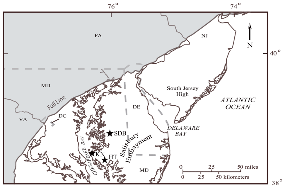
Figure 1Map showing the location of Knapps Narrows (KN), the South Dover Bridge (SDB), and Howards Tract (HT) coreholes. The Fall Line delimits the crystalline basement rock (gray) from Cretaceous–Cenozoic-age coastal plain sediments (white). Modified from Self-Trail et al. (2017b).
2.2 Methods
2.2.1 Nannofossil biostratigraphy
The calcareous nannofossil biozonation was established, and core descriptions were made in the field and at the U.S. Geological Survey (USGS) Florence Bascom Geoscience Center. A total of 42 samples, taken at approximately 0.15 m intervals for calcareous nannofossil analysis, were extracted from the center of freshly broken core to avoid contamination from drilling fluid. Smear slides for calcareous nannofossil analysis were prepared using the standard technique of Bown and Young (1998), combined with the double-slurry technique of Blair and Watkins (2009) and mounted using Norland Optical Adhesive 61. Slides were examined under cross-polarized light, using a Zeiss Axioplan 2 light microscope (LM) at 1250× magnification. Biostratigraphic zones were based on the NP zonation of Martini (1971) and supplemented by the biohorizons of Agnini et al. (2014). Smear slides are housed in the USGS calcareous nannofossil laboratory in Reston, VA.
2.2.2 Paleomagnetism
Paleomagnetic data were generated at the Paleomagnetism Lab of Lehigh University. A total of ∼ 100 minicores were collected from the Knapps Narrows core (40–110 m), with sampling spacing of 0.2 to 1.5 m guided by preliminary biostratigraphic constraints. Stepwise thermal demagnetization in an ASC Model TD48-SC thermal demagnetizer was applied to the samples, followed by measurement on a three-axis 2G Enterprises 755 superconducting rock magnetometer. Heating involved at least seven treatments, at ∼ 25 ∘C/50 ∘C steps from 100 to 350 ∘C for the weak samples and up to 575–600 ∘C for stronger ones. Thermal demagnetization generally ceased when the remanent magnetization displayed anomalous surges in magnetization, was too weak for magnetometer precision, or exhibited irregular magnetic directions and/or intensities for two or three consecutive steps. The choice of a thermal rather than an AF (alternating field) demagnetization procedure was due to the potential existence of high-coercivity magnetic minerals (e.g., goethite).
Samples from rotary cores may have been shifted from their original declination orientation. The overprint components from drilling-induced magnetization and from normal-polarity, present-day (late Quaternary) field remanence are observed and could often be easily removed during initial demagnetization steps. Instead, normal (N) or reversed (R) polarity could be indicated by natural remnant magnetization (NRM), which pointed downward (N) or upward (R). The present-day magnetic field direction is −11.11∘ declination and 64.88∘ inclination (from https://www.ngdc.noaa.gov/geomag-web/#igrfwmm, last access: 10 August 2023, for the modern Knapps Narrows core location), which should be roughly the same as the Eocene, since no major continental movement has occurred (Scotese, 2014).
Polarity zones were assigned to stratigraphic clusters of good-quality characteristic remanent magnetization (ChRM) vectors, while uncertain intervals were assigned to clusters of noisy magnetic behaviors and to significant gaps in the sampling coverage (Przybylski et al., 2010). Detailed paleomagnetic data and additional data analysis protocol are available in the supplementary paleomagnetism Microsoft Excel workbook (see the “Data availability” section).
Given that sediments are largely semi-consolidated, a non-magnetic plastic tube was inserted in the core to extract a sediment plug. The plug was then extruded into aluminum foil pieces and tightly wrapped. Occasionally, paleomagnetic samples were taken by pushing non-magnetic cubes directly into the center of the core halves so that alternate field demagnetization could be used.
The interpreted polarity and characteristic directions of the samples were given a quality rating of “N(R)”, “NP(RP)”, “NPP(RPP)”, “N?(R?)”, or “INT” to samples yielding definite to uncertain ChRM directions, according to a semi-subjective judgment of the behavior of the magnetic vectors during the stepwise demagnetization. This quality rating helps to define a more accurate magnetostratigraphy (Zhang and Ogg, 2003). The N or R ratings were generally assigned to those samples that attained a (semi-)stable endpoint direction (characteristic remanent magnetization or ChRM) during progressive demagnetization. However, only a small subset of our samples displayed this ideal resolution of primary magnetization. We applied a “P” tag of RP or NP when the residual magnetization vector was considered close to attaining an endpoint before losing its residual magnetization or experiencing a surge. The “PP” tag was applied to samples that had a distinct trend toward the polarity hemisphere, which was considered to be indicative of the underlying polarity but also considered to be too far from attaining an endpoint before dying to be used in statistics for computing a mean direction. The “?” qualifier was used to denote possible trends toward an underlying polarity, and INT is for classifying elements that were either entirely uncertain or displayed an endpoint that was intermediate between the N and R poles. Polarity zones were assigned to stratigraphic clusters of ChRM vectors rated as N-NP-NPP or R-RP-RPP. Uncertain intervals were assigned to clusters of N?-INT-R? and to significant gaps in sampling coverage. Summary plots of the lithology of the Knapps Narrows with the interpreted polarity patterns (Fig. A2) were generated with the public TS-Creator database and visualization software (https://timescalecreator.org, last access: 10 August 2023).
2.2.3 Bulk isotope stratigraphy and age model
Bulk carbonate content and bulk carbonate and benthic foraminiferal stable carbon and oxygen isotope analysis was performed in the Earth and Planetary Sciences Department at the University of California, Santa Cruz. CaCO3 content was determined using a UIC CM140 coulometer. In this system, approximately 20 mg of sediment is dissolved in 2N sulfuric acid. For isotope analyses of bulk carbonate, a mass of ground sediment was weighed to obtain between 35 and 50 µg of carbonate. All samples were analyzed with a Kiel IV carbonate device paired with a Thermo Scientific MAT253 mass spectrometer. The analytical precision of this system, based on replicate analyses of Carrara marble standards, is better than 0.05 ‰ for carbon isotopes.
An age model was constructed for this section on the basis of carbon isotope stratigraphy, specifically the carbon isotope excursion (CIE) minima and maxima (respectively, H1 and H2), correlated to the orbitally tuned deep ocean records of Lauretano et al. (2015). This age model was then used to calculate sedimentation rates.
2.2.4 Spectral analysis
Spectral analysis (eCOCO or evolutionary correlation coefficient) of the gamma ray wireline log of the cored interval was performed via Acycle v2.4.1 to obtain an estimate of the sedimentation rate variations (Li et al., 2019). The eCOCO analysis computes the correlation coefficient (COCO; ρ) between the frequency spectra of target astronomical solutions and the presence of different cycles within studied data, which provides the numerical estimation of the optimal depositional rates (a higher correlation coefficient corresponds to the most likely sedimentation rates) within a sedimentary record (Li et al., 2018, 2019). Monte Carlo simulations are embedded in the COCO method to test the significant level of astronomical forcing assumption.
2.2.5 Palynology
In total, 18 samples were processed at Utrecht University for quantitative palynological analysis. Between 3 and 15 g of freeze-dried, lightly crushed sediment was spiked with a known number of exotic Lycopodium spores and subsequently treated once with 30 % HCl and twice with ∼ 38 %–40 % HF to dissolve carbonates and silicates, respectively. The insoluble residue was sieved using 15 and 250 µm nylon mesh sieves, with ultrasonic bath steps to break up the agglutinated organic matter. The resulting 15–250 µm palynomorph fraction was mounted on glass microscope slides. A general characterization of palynofacies, palynomorph categories (pollen, spores, and aquatic algae), and dinocysts in particular was performed with light microscopy (typically 630× magnification or 1000× magnification, when required), counting at least 200 and typically > 250 elements. For taxonomy, we refer to that cited in Williams et al. (2017), with the exception of wetzelielloid taxa (see Bijl et al., 2017). For paleoecological reconstructions, dinocyst taxa are grouped in complexes of morphologically related species and genera with assumed similar paleoecological affinities, following the empirically based complexes of Frieling and Sluijs (2018).
2.2.6 Clay mineral analysis
Clay mineral analysis was performed in the Earth and Planetary Sciences Department at the University of California, Santa Cruz. Methods were adapted from Kemp et al. (2016), Gibson et al. (2000), and Poppe et al. (2001). Samples were gently crushed and placed in a 1 % sodium hexametaphosphate (Calgon) solution adjusted to a pH of 7–7.5 via the addition of ammonium hydroxide. Samples were disaggregated by placing them on a shaker table at approximately 200 rpm (revolutions per minute) for 48 h. Samples were then wet-washed through a 63 µm sieve to separate the coarse and fine fraction. Samples were then marked 5 cm from the surface of the solution and shaken to resuspend the clay minerals. The suspension was allowed to settle for 4:06 h at 20 ∘C, in accordance with Stoke's law. The suspension above the 5 cm mark was then extracted via syringe to isolate the < 2 µm size fraction. This suspension was then dried, and approximately 150 mg of this clay-sized fraction was then resuspended in deionized water. The suspension was then passed through a submicron filter attached to a vacuum apparatus to remove the water and orient the clays. The filter paper was removed and placed on the side of a glass beaker before being transferred to a glass slide to produce an oriented mount. For the glycolation step, mounts were placed inside a desiccation chamber with ethylene glycol at 60 ∘C for a minimum of 4 h.
Oriented mounts were scanned in a Philips 3040/60 X'Pert Pro X-ray diffraction unit from 0–35∘ 2θ, with a 1∘ source beam and a ∘ receiving slit at 45 mA and 40 mV. The results were then printed, and individual sample peaks were weighed to provide a semi-quantitative measurement of clay mineral abundances.
2.2.7 Foraminifer oxygen isotope paleothermometry
Temperatures based on benthic foraminiferal oxygen isotopes ratios were estimated, following the protocol outlined in Hollis et al. (2019). The paleotemperature equation of Marchitto et al. (2014) was used. Then, four to six Anomalinoides acutus specimens were picked from the 180–250 µm size fraction at each interval. All samples were analyzed with a Kiel IV carbonate device paired with a Thermo Scientific MAT253 mass spectrometer. The analytical precision of this system, based on replicate analyses of Carrara marble standards, is better than 0.05 ‰ and 0.10 ‰ for δ13C and δ18O, respectively. In order to calculate an absolute temperature, bottom δ18OSW was estimated based on the relationship between the salinity and δ18O established by Fairbanks (1982) and the modern-day salinity measurements reported in Richaud et al. (2016), with a −1.2 ‰ correction applied to account for the lack of ice during the early Eocene.
2.2.8 TEX86 biomarker paleothermometry
TEX86 analysis was performed on 18 samples at Utrecht University. Glycerol dialkyl glycerol tetraether (GDGT) lipids were extracted from ∼ 10 g of powdered, freeze-dried sediment in 25 mL solvent mixture of dicholormethane (DCM) : methanol (MeOH) (9:1; ) by a Milestone ETHOS X microwave extraction system, which was set to 70 ∘C for 50 min. Filtered (using NaSO4 column) total lipid extracts were dried and separated into apolar, neutral, and polar fractions through AlOx column chromatography, with hexane DCM (9:1), hexane DCM (1:1), and 1:1 DCM MeOH (1:1), respectively, as mobile phases,; thereafter, the extracts were dried again and weighed. Polar fractions, after the addition of a GDGT standard (99 ng of 744) for quantitative analyses, were diluted in hexane isopropanol (99:1) to a concentration of 2 mg mL−1. A 10 µl aliquot was filtered (0.45 µm polytetrafluoroethylene) and analyzed by high-performance liquid chromatography (HPLC) coupled to an ionization mass spectrometer. The analytical precision was 0.006 TEX86 units, determined using an in-house GDGT standard. We use several indices to constrain potential confounding effects, such as GDGT contributions from methanogenic/methanotrophic microorganisms, terrestrial sources, and deepwater archaea. TEX86 values were calculated from isoprenoid GDGT abundances, following Schouten et al. (2002), and converted to sea surface temperature (SST) using linear and exponential calibrations (e.g., Kim et al., 2010; O'Brien et al., 2017), following recommendations by Hollis et al. (2019). Calibration errors are on the order of ±2.5 ∘C (1 SD), but any offset from this calibration is assumed to be a constant throughout the study section.
3.1 Stratigraphic framework
A distinct magnetic reversal pattern is preserved in the Knapps Narrows core, with the section below 99.21 m (sample KN37) exhibiting a reversed polarity and the upper section (above 91 m, sample KN36) a normal polarity. The reversal boundary, identified as the transition from magnetochron C24r to C24n based on nannoplankton stratigraphic data, thus lies within 99.21–91 m (Fig. 2). The lowermost section is placed in zone NP10, based on the first occurrence (FO) of Rhomboaster spp. and the absence of Tribrachiatus contortus, which has its FO at 96.6 m. The top of zone NP10 is placed at 95.2 m on the last occurrence of T. contortus, and the base of zone NP11 is identified at 95.1 m, based on the FO of T. orthostylus. This reconstructed bio-magnetostratigraphy (Figs. A2 and A3) is generally consistent with the Paleogene timescale 2020 (Speijer et al., 2020) and the timing of ETM2 (Cramer et al., 2003; Lourens et al., 2005; Westerhold et al., 2007; Stassen et al., 2012a).
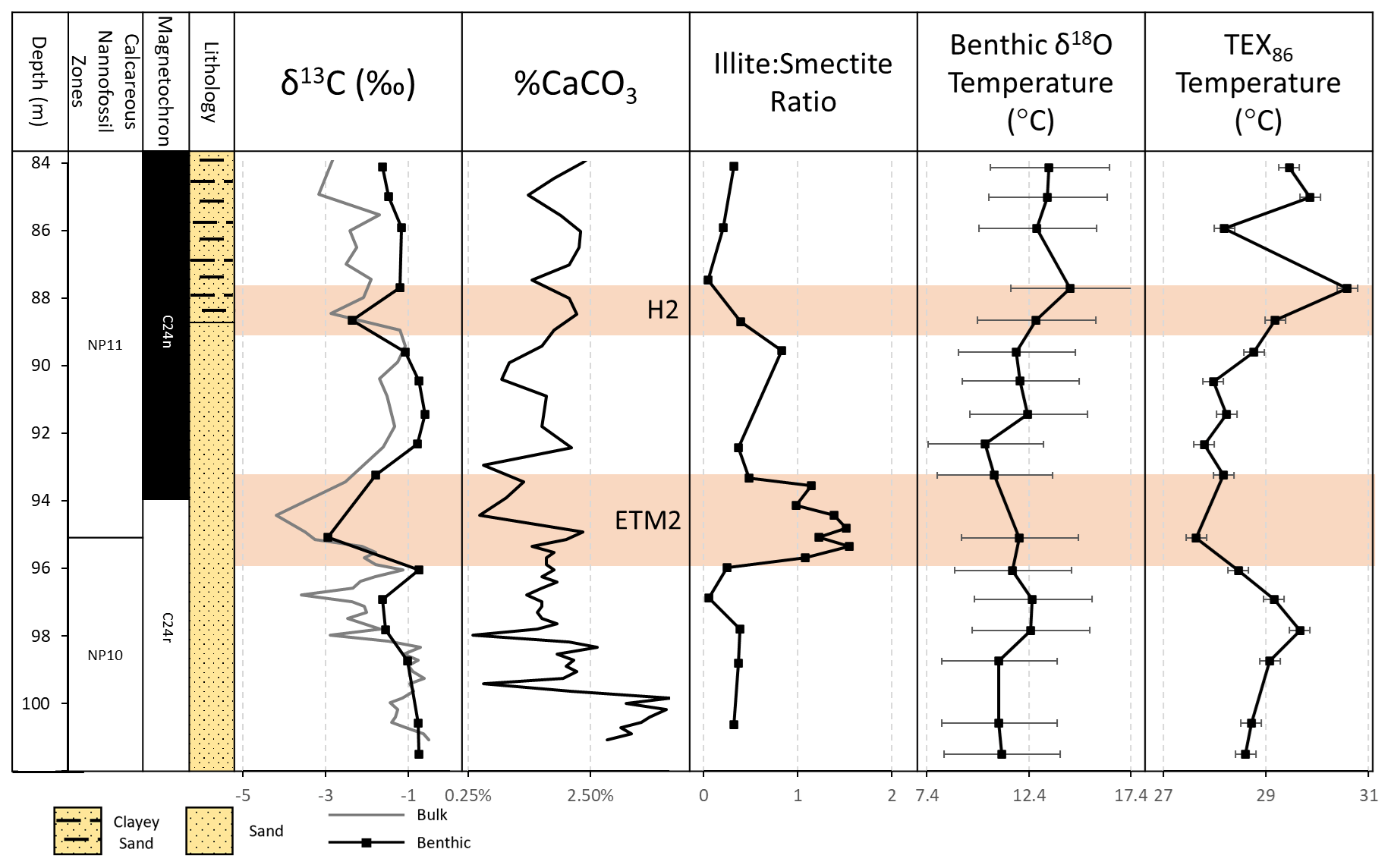
Figure 2Knapps Narrows core site (from left to right) depth, nannofossil zones, magnetochrons, lithology, carbon isotopes, percent carbonate, clay mineralogy, and benthic δ18O temperatures, as well as the TEX86 sea surface temperatures over the ETM2 and H2 interval at Knapps Narrows. TEX86 temperatures use linear calibration from O'Brien et al. (2017). The error in δ18O represents 1 PSU change in salinity. Note the logarithmic scale for percent carbonate and low-carbonate interval at ETM2, spike in the illite–smectite ratio at ETM2, agreement between benthic and sea surface temperatures, and offsets in timing between carbon isotopes, clay mineralogy, and temperature proxies.
The bulk carbonate δ13C record captures a −1.5 ‰ excursion from 98.18–96.41 m before recovering to the baseline, followed by a second −2.5 ‰ excursion between 95.37–93.46 m that peaks at 94.48 m (Fig. 3). This double-peak feature facilitates the recognition of ETM2, as it is documented for several marine and continental sections (e.g., Walvis Ridge and Bighorn Basin in Fig. 3; Cramer et al., 2003; Stap et al., 2010; Abels et al., 2016). Between 93.46 and 88.98 m, the carbon isotope ratios return to near-baseline values before another −1.5 ‰ excursion at 88.51 m, consistent with observations of H2 at other sites (Fig. 3; Cramer et al., 2003; Stap et al., 2010; Abels et al., 2016). Benthic foraminiferal carbon isotope trends largely track those in bulk carbonate. An interval with low-carbonate content (∼ 93–94.5 m; Fig. 2) coincides with the CIE minima at 94.48 m, where the sediments were barren of foraminifera.
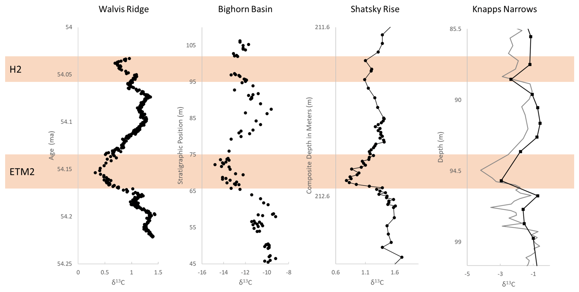
Figure 3Carbonate δ13C records of ETM2 and H2 at Walvis Ridge (bulk), Bighorn Basin (pedogenic nodules), Shatsky Rise (benthic), and Knapps Narrows (this study). For Knapps Narrows, bulk carbonate values are in gray, and benthic values are in black. Knapps Narrows at 94.5 m was nearly barren of foraminifera. Walvis Ridge data are from Stap et al. (2010), the age model is from Lauretano et al. (2015), Bighorn Basin data are from Abels et al. (2016), and Shatsky Rise data are from Westerhold et al. (2018).
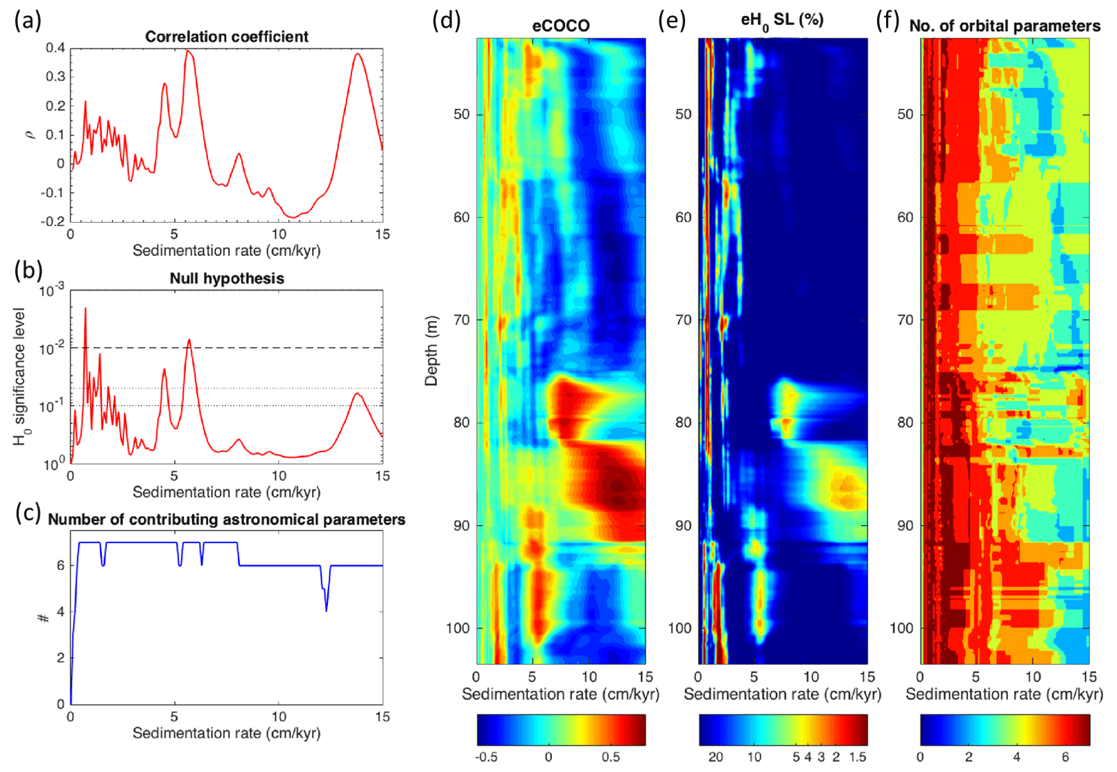
Figure 4COCO (a–c) and eCOCO (d–f)analysis of the wireline gamma ray log (42.5–103.5 m). The studied interval lies between 84 and 102 m. In the COCO plots, three clusters of high-ρ sedimentation rates, accompanied with a low-H0 significance level, and relatively more (6–7 parameters) contributing astronomical parameters are identified, i.e., at ∼ 1, ∼ 5, and ∼ 13 cm kyr−1. For the eCOCO analysis, the sliding window is 18 m, using 0.2 m steps. The target astronomical solution is La2004 at 53 Ma (with seven astronomical cycles at 405, 125, 95, 39.2, 23.1, 21.9, and 18.8 kyr, respectively). All periodograms were analyzed, with the autoregressive (AR1) red noise model removed. The number of Monte Carlo simulations is 2000. The tested sedimentation rates range from 0 to 15 cm kyr−1, with a time step of 0.1 cm kyr−1. Note that from depths of ∼ 82–90 m, which cover the studied interval, a change in the sedimentation rate exists from ∼ 5 to ∼ 13 cm kyr−1. The evolutionary power spectrum (Fig. A5) of this interval also indicates a distortion of cyclicity.
The COCO and eCOCO (Fig. 4) analysis shows a sedimentation rate of ∼ 5 cm kyr−1 for most of the succession from 103.5 to 43.5 m, except for the interval of 90 to ∼ 82 m, where there is a transition to a sedimentation rate of approximately 13 cm kyr−1. Assuming orbital forcing, the ∼ 5 cm kyr−1 and a cycle of ∼ 18 m (Fig. A5) correlates to the 405 kyr long eccentricity period. Given the surge in estimated sedimentation rate, the observed ∼ 18 m cycle should instead correlate to the short eccentricity periodicity. Given the sudden increase in deposition rate, this interval may reflect on other factors; for example, there could be a period of enhanced precipitation, even though this period of elevated sedimentation rates does not correspond to any hyperthermal event, or bathymetric changes related to regional faulting.
3.2 Palynology
Palynological associations are dominated by marine palynomorphs, notably dinocysts, and are common to abundant organic linings of benthic foraminifera. Terrestrial palynomorphs such as pollen and spores are rare. Dinocyst assemblages are well preserved and diverse. They comprise a typical mid–early Eocene shelf assemblage, given the abundant contributions of Spiniferites spp., Operculodinium spp., and species grouped in the Areoligera and Cordosphaeridium complexes (e.g., Pross and Brinkhuis, 2005; Frieling and Sluijs, 2018). The distribution pattern of various chronostratigraphic index taxa such as Biconodinium longissimum and several wetzelielloids (e.g., W. articulata and W. tabulatum) further confirm the assignment to ETM2 and H2 (e.g., Williams et al.,2004; Bijl, 2022). The Senegalinium complex, particularly abundant in the lower part of the section, tolerated low salinities, which is suggestive of strong seasonal river runoff and is in apparent contradiction to the absence of terrestrial pollen and spores (Brinkhuis et al., 2006; Sluijs and Brinkhuis, 2009).
3.3 Clay mineralogy
Clay mineralogy shows moderate variation throughout the studied interval. The clay size fraction is dominated by smectite (> 50 % and up to 95 %) over much of the studied interval, with the remainder being composed largely of illite. There is a marked increase in illite during the body of ETM2, which peaks at a 1.5 illite smectite ratio, and an additional, smaller, increase in the illite smectite ratio immediately prior to H2 (Fig. 2). There is no detectable kaolinite within the studied interval. These variations are not correlated with other proxies, and the timing of the mineralogic changes is offset relative to the CIEs of ETM2 and H2; i.e., the shift in mineralogy begins prior to the CIE of ETM2 and after the CIE of H2.
3.4 Oxygen isotope paleothermometry
There is a long-term rise in temperature over the studied interval from 11.1 ∘C () at the base of the core to 13.4 ∘C () at the top (Fig. 2). The largest source of error associated with the δ18O temperature measurements is the uncertainty associated with local δ18OSW. According to the Fairbanks (1982) equation, a change in salinity of ±1 PSU, when propagated across calculations, can result in an error in the temperature on the order of ±2.9 ∘C, depending on the local freshwater δ18O. This error cannot be assumed to be constant throughout the core, as hydroclimate is expected to change dramatically during this time period, which could impact local salinity and often seems to be the case with the PETM. Agreement in temperature trends between δ18O and TEX86 suggests that this effect is minimal. Bottom water temperatures during ETM2 were measured to be 11.6 ∘C (), which is 0.9 ∘C warmer than the baseline value. The greatest warming is seen following the CIE associated with H2 at 14.4 ∘C (), which is 2.3 ∘C warmer than the baseline. Peak warming seems decoupled from minimum δ13C values for both ETM2 and H2 (Fig. 2). These temperature variations are likely the minimum estimates given the resolution of the record.
3.5 TEX86 biomarker paleothermometry
SST values based on TEX86 vary by a few degrees, largely mirroring the benthic bottom water temperature trends (Fig. 2). TEX86 records for this site indicate a warming on the order of 3–5 ∘C over the studied interval. Temperatures appear to increase prior to the body of ETM2 during the pre-onset excursion. Using a linear calibration, SST reached a maximum of ∼ 30 ∘C, which is ∼ 1.1 ∘C higher than the baseline. Exponential calibrations result in slightly lower SSTs and slightly muted warming (see the “Data availability” for more information). TEX86 reaches minimum values during the CIE associated with ETM2 at ∼ 28 ∘C, which 1.0 ∘C colder than baseline values. The trend reverses and reaches a maximum, following the CIE associated with H2 at ∼ 31∘C, which is ∼ 1.3 ∘C warmer than the baseline value.
4.1 Stratigraphy and sedimentation
Documented sections spanning the ETM2 in marine shelf settings are rare compared to those spanning the PETM. The discovery of the lithologic expression of two smaller hyperthermals, ETM2 and H2, in addition to the PETM, on the mid-Atlantic coast provides a unique opportunity to assess how regional climate responded to two distinct levels of greenhouse forcing. Apart from bio-magnetostratigraphy, the key to identifying ETM2 is the stable carbon isotope stratigraphy, specifically the presence of the paired CIEs of ETM2 and H2, which, at Knapps Narrows, is broadly consistent with trends observed elsewhere (Fig. 1). The magnitude of the CIE here is intermediate compared to records of the ETM2 in open-marine and continental settings but is consistent with observations of the PETM CIE in marginal marine settings (John et al., 2008; Tipple et al., 2011; Sluijs and Dickens, 2012). The marine carbonates of ETM2 document a smaller excursion than those observed in continental sections and in marine organic carbon (Tipple et al., 2011; Stap et al., 2010; Westerhold et al., 2018; Abels et al., 2016; Sluijs and Dickens, 2012). The dampening of the magnitude of change in marine carbonates has been attributed to dissolution and carbonate chemistry changes during the peak of the hyperthermal (e.g., PETM). The enhanced terrestrial signal has been attributed to changes in soil conditions, humidity, plant communities and physiology, and an increase in the organic 13C fraction (Bowen et al., 2004; Tipple et al., 2011; Sluijs and Dickens, 2012). The relative lack of dissolution in shallower marine environments and lack of controls that enhance the terrestrial signal likely contribute to this more intermediate CIE.
Although the interval with low-carbonate content prevented the generation of a more detailed foraminiferal isotope record, the covariance between bulk carbonate and benthic foraminiferal δ13C throughout, combined with the biostratigraphy and magnetostratigraphy, confirms our interpretation of the carbon isotope stratigraphy. The onset of the PETM in the mid-Atlantic region is characterized by a clay or low-carbonate layer, which has been attributed to both coastal acidification and enhanced siliciclastic sediment fluxes that are climatically driven (Bralower et al., 2018; Gibson et al., 2000; Kopp et al., 2009). High-resolution climate simulations are consistent with enhanced seasonal or peak precipitation, which likely increased the rates of erosion and sedimentation (Carmichael et al., 2017; Rush et al., 2021). Similarly, there are two potential explanations for the low-carbonate interval associated with the body of ETM2, namely coastal acidification and enhanced siliciclastic flux. Coastal acidification would inhibit the calcification and potentially dissolve carbonate directly, leading to the low-carbonate interval. In arguing for increased acidification, Bralower et al. (2018) put forth two possibilities, namely a possible shoaling of the lysocline to the middle shelf and a regional shoaling of the lysocline driven by enhanced eutrophication and microbial activity. However, the increase in pCO2 levels during ETM2 was much lower than that of the PETM (e.g., Harper et al., 2020), and there is little evidence for a global shoaling of the lysocline to this degree during ETM2. Therefore, it is unlikely that elevated CO2 levels alone could drive dissolution on the shelf in this region, given the rates of estimated C emissions. It is possible that dissolution could be enhanced by increased oxidation of organic matter for both in situ organic matter and organic matter transported into the shelf (Bralower et al., 2018; Lyons et al., 2019). However, the dinoflagellates in our study interval do not suggest significant changes in productivity in response to the CIEs. Enhanced siliciclastic transport may have contributed to the low-carbonate interval as well, even though this increase appears to be to a much lesser extent relative to the PETM with an estimated 50 %–100 % increase in supply rates within the studied interval, as compared to estimates of 2.8 to 220-fold increases within the PETM. Again, the inflection occurs at ∼ 92 m whereupon the sedimentation rate increase is not correlated to either hyperthermal (Stassen et al., 2012b), although recent studies have suggested much more moderate increases in sedimentation rates across the PETM, which is in good agreement with observations here (Li et al., 2022). Lacking a clear indication of a single driver for the low-carbonate interval, it is likely that a confluence of factors drove the observed changes.
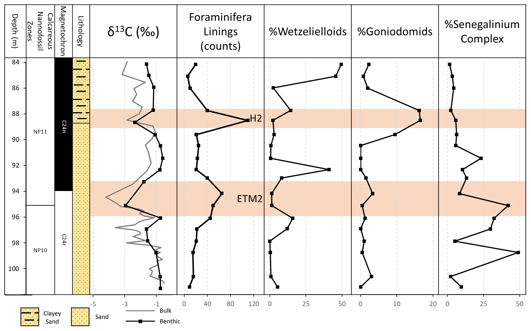
Figure 5Knapps Narrows core site (from left to right) depth, nannofossil zones, magnetochrons, lithology, carbon isotopes, foraminifera lining counts, relative abundance of wetzelielloids, relative abundance of Goniodomids, and relative abundance of the Senegalinium complex. Foraminifera linings can be used to infer periods of rapid or low siliciclastic influx. Wetzelielloids are associated with periods of high productivity, Goniodomids are associated with high temperatures and strong salinity stratification, and the Senegalinium complex is associated with low salinity (Frieling and Sluijs, 2018). Of note is a long-term increase in salinity from relatively fresh conditions at the base of the core to more saline conditions upsection. Rapid changes in the abundance of wetzelielloids suggest disconformities, periods of non-deposition, or condensed sections.
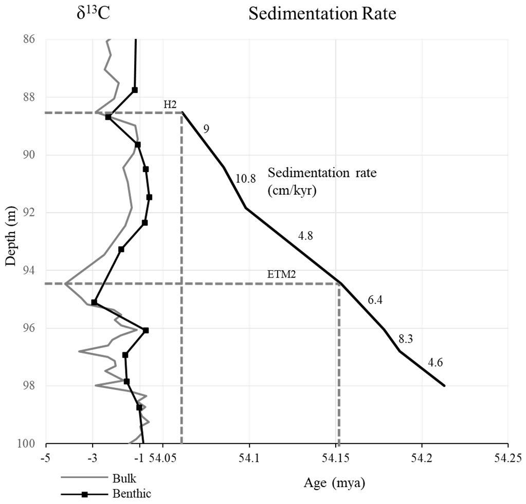
Figure 6Sedimentation rates in the Knapps Narrows core based on the correlations of δ13C inflection points to the age model of Lauretano et al. (2015) at Walvis Ridge site 391. Sedimentation rates are given in centimeters per thousand years. Note the relative consistency compared to the order of magnitude changes that were documented during the PETM in Stassen et al. (2012b), with moderate increases beginning at 91.8 m, which is consistent with cyclostratigraphy.
Although the coarse resolution of the carbon isotope stratigraphy might not capture a brief increase in sedimentation rates, our age model indicates that the sedimentation rates remained fairly constant across ETM2 and H2, which is in contrast to the lithologic expression of the PETM in this area. Assuming continuous sedimentation, rates range from 4.6 to 10.8 cm kyr−1, with the lower section of the core trending lower and the upper section of the studied interval trending higher, with an inflection point at 91.8 m. The lowest rates occurred prior to ETM2, and the highest occurred during the background state between ETM2 and H2 (Fig. 6). However, sedimentation rates in shelf settings can vary on timescales shorter than the resolution of our age model is able to detect. It is almost certain that the records reflect the amalgamation of periods of enhanced sedimentation and non-deposition (Trampush and Hajek, 2017). Abrupt transitions within the distribution patterns of several dinocyst species suggest minor disconformities, condensed intervals, or depositional hiatuses that would result in highly variable sedimentation rates that we cannot record, based on the resolution of our carbon isotope age model. Therefore, the age model should be seen to be capturing the average over long time periods.
The sedimentation rates predicted based upon the age model are largely consistent with those calculated based on spectral analysis, which found long-term average sedimentation rates on the order of 5 cm kyr−1 in the lower section of the core and 13 cm kyr−1 in the upper section, with an inflection point at the same location as predicted by the age model at ∼ 92 m (Fig. 4). Based on spectral characteristics, the lower section of the core exhibits cyclicity that could be orbitally paced, while the upper section does not. This is unsurprising, given the generally discontinuous or episodic nature of sediment accumulation in such facies. Despite the aforementioned issues surrounding the stochastic nature of shelf deposition, Cyclostratigraphic methods have been used in calculating shelf sedimentation rates for the PETM in the region, and the general agreement between the carbon isotope record and the spectral analysis suggests the general interpretation of a bimodal sedimentation pattern is accurate (Li et al., 2022).
Other factors may have a role in observed sedimentation rates, such as the paleobathymetry and local sea level. Faulting within the region could have led to the development of horst and graben complexes (Fig. A1). These positive and negative structural features could produce localized paleobathymetric highs and lows that could have influenced the observed variation in local sedimentation rates (Sabat, 1977; Self-Trail et al., 2017a).
4.2 Regional hydrology and depositional setting
Evidence supporting a modest intensification of the hydrologic cycle includes the shift in clay mineralogy from smectite-dominated facies to illite-dominated facies during the body of ETM2 and a moderate increase in illite prior to H2, with no detectable levels of kaolinite. Clay mineralogy is used extensively as a proxy for chemical weathering, with a spectrum from smectite and illite to kaolinite being associated with increasingly wet and warm conditions (Singer, 1980). Many locations experience a dramatic increase in kaolinite during the PETM (Robert and Kennett, 1994; Gibson et al., 2000; Kemp et al., 2016; Chen et al., 2016). Previous studies on clay mineralogy over the PETM in the Salisbury Embayment demonstrated that kaolinite increased and that this increase could have resulted from the reworking of older deposits (Gibson, 2000; John et al., 2012). In other regions, the increase in kaolinite is believed to result from an authigenic weathering response to the PETM (Clechenko et al., 2007; Chen et al., 2016). Work on the radioisotopes of the clay minerals, namely strontium and lead, demonstrate little change in the sourcing of sediment in the Atlantic Coastal Plain during the PETM, and work on lithium isotopes seems to suggest rapid changes to global weathering patterns during the PETM (Rush et al., unpublished data; Pogge von Strandmann et al., 2021; Ramos et al., 2022). Since illite is a product of weathering between smectite and kaolinite, alongside recent studies demonstrating an immediate weathering response during the PETM, its presence seems to support the interpretation that the clays formed in situ during ETM2. As the warming of ETM2 is intermediate to that of the background state and the PETM, the environmental perturbations during ETM2 would likely illicit a weathering response intermediate to the background state and that of the PETM.
The palynological assemblages imply a complicated story. The assemblages are typical of those seen in neritic settings (Pross and Brinkhuis, 2005; Frieling and Sluijs, 2018). They show a large degree of variability in freshwater runoff, stratification, and productivity, but the majority of these changes show no relation to δ13C or temperature change, which is atypical for dinocysts (Fig. 5). Wetzelielloids, which include the Apectodinium complex and Apectodinium spp., show (quasi-)global abundance peaks across the PETM but demonstrate a small relative increase prior to ETM2, with their highest relative abundances occurring several meters above both ETM2 and H2 (Crouch et al., 2003; Frieling and Sluijs, 2018; Fig. 5). The only anomaly that clearly corresponds to a hyperthermal is the peak abundance of Goniodomideae during H2 (Fig. 5). Goniodomideae represent a thermophile group thriving in lagoonal environments (variable salinity) and further offshore under strongly stratified conditions (e.g., Reichart and Brinkhuis, 2003; Frieling and Sluijs, 2018). Taking into account the decreasing abundance of the Senegalinium complex, this likely points to an increase in salinization during this interval, due to decreased runoff or increased evaporation. This interval also yields anomalous abundances of benthic foraminifer linings, which generally indicate a temporary reduction in sedimentation, further supporting the interpretation of decreased runoff during this interval.
An overall shallowing trend in the upper section of the core may be inferred, based on a long-term decline in the abundance of the low-salinity-tolerant Senegalinium complex and a rise of the Goniodomids, which typically occur in massive (harmful) blooms in (seasonally) high-salinity, warm, lagoonal conditions in modern and ancient settings (Zonneveld et al., 2013; Frieling and Sluijs, 2018; Sluijs et al., 2018). This shallowing trend also indicates a shift from brackish conditions to more saline conditions upsection that do not necessarily correspond to hyperthermal events and may indicate an overall longer-term trend.
Increased abundances of the low-salinity-tolerant Senegalinium complex and the supply of terrestrial palynomorphs suggest increased river runoff in shelf sections across hyperthermal events (e.g., Crouch et al., 2003; Sluijs and Brinkhuis, 2009; Sluijs et al., 2009). These abundances in Knapps Narrows show no correspondence to the CIEs or temperature anomalies. The complex was abundant before, during, and after ETM2 but was not present during H2 after its gradual decline, which does not support a strong hydrological response to this event. Terrestrial palynomorphs are rare throughout the record, reminiscent of the upper Paleocene and lower Eocene of the New Jersey Shelf (e.g., Zachos et al., 2006). This suggests changes in transport of terrestrial palynomorphs or that the hinterland was sparsely vegetated in the region, also explaining the lack of response during the PETM, ETM2, and H2 (Self-Trail et al., 2017b). This may be consistent with the paleolatitude of about 33∘ N (http://www.paleolatitude.org/, version 2.1, last access: 10 August 2023; van Hinsbergen et al., 2015), which arguably would represent an arid zone. Quantitative reconstructions of salinity could aid in this interpretation. However, at present, we are unable to reconstruct surface salinities due to a paucity of surface-dwelling foraminifera species within the studied interval and the qualitative nature of dinoflagellate-based paleoenvironmental reconstructions.
Goniodomids reach a maximum at H2 that also corresponds to the highest reconstructed temperatures. A rise in salinity seems to precede this warming, but it should be noted that dinoflagellate blooms are strongly seasonal and therefore should not necessarily correspond to our salinity estimates. The correspondence of Goniodomid abundances with transient global warming events has been previously recorded, for example, in brief intervals of the PETM on the New Jersey Shelf, the Nigerian Shelf, and across the middle Eocene climatic optimum in the eastern equatorial Atlantic (Sluijs and Brinkhuis, 2009; Frieling et al., 2017; Cramwinckel et al., 2019). Very high stable carbon isotope ratios suggest that these Goniodomid abundances indicate that at least some of these abundances represent an increase in the geographical range and frequency of harmful blooms (Frieling et al., 2017; Sluijs et al., 2018).
In contrast to the records here, the Lomonosov Ridge palynological assemblages demonstrate a marked shift during ETM2, with an increase in dinoflagellate markers that are indicative of freshening and eutrophication and the appearance of palm pollen that indicates high winter temperatures (Sluijs et al., 2009; Willard et al., 2019). Further evidence of hydrologic changes is noted in the hydrogen isotope records of leaf wax n-alkanes, which demonstrate a large rise during the PETM, a rise prior to ETM2, and a drop during the body of the event, as well as during H2 (Pagani et al., 2006; Krishnan et al., 2014).
Looking at other trackers of hydrologic changes across hyperthermals, records of enhanced siliciclastic flux were archived at Mead and Dee streams in Aotearoa / New Zealand across several hyperthermal events (Nicolo et al., 2007; Slotnick et al., 2012). While focused more on biotic and ocean chemistry conditions, the Nile Basin is also interpreted as having a similar response to the PETM but on a smaller scale (Stassen et al., 2012a). Such evidence of enhanced hydrology driving siliciclastic fluxes is also found in hemipelagic sections such as the Terche section of northeastern Italy (D'Onofrio et al., 2016).
The records from continental sections suggest that changes in the regional precipitation patterns were not entirely uniform. An increase in siliciclastic sediment flux in a terrestrial section at Ellesmere Island is interpreted as evidence of an intensified hydrologic system during ETM2 (Reinhardt et al., 2022). The Bighorn Basin record suggests contrasting regional climatic changes between the PETM and later hyperthermal events (Abels et al., 2016), which is in line with observations from this study.
The overall hydrologic response to ETM2 appears much more modest than that of the PETM and somewhat muted, given the scale of global warming and assuming a roughly linear response of precipitation patterns to global warming. Given that the baseline temperature prior to ETM2 is a few degrees higher than prior to the PETM, it is possible that sensitivity to an equivalent temperature perturbation would be less extreme than for the PETM, i.e., a state-dependent response. This also suggests variability in the hydroclimate responses to greenhouse forcing in different regions. While the Arctic records demonstrate a strong hydrological response across ETM2, here the interpretation is less straightforward (Sluijs et al., 2009). Depending on the region, the local hydroclimate seems to respond in a somewhat non-linear fashion to global warming, characterized more by abrupt mode shifts (e.g., frequency of extremes or duration of wet vs. dry seasons), as opposed to gradational changes (e.g., mean annual precipitation; Carmichael et al., 2017; Rush et al., 2021). In the mid-Atlantic region, our palynological record appears to confirm this overall mild response to the ETM2. In effect, to record only minor changes is rather unique, given that other transient climatic events in the Cenozoic are typically characterized by massive concomitant dinocyst assemblage changes and more significant changes in sedimentation.
4.3 Temperature
GDGT distributions indicate a dominant pelagic thaumarchaeotal source based on low abundances of terrestrial GDGTs and of lipids derived from methanotrophs or methanogenetic microorganisms (Fig. A3). GDGT2 3 ratios between 1.6 and 2.1 (Fig. A4) indicate a dominant lipid origin from the upper ∼ 150 m of the water column (Hurley et al., 2018; van der Weijst et al., 2022). Although this may imply contributions from sub-thermocline Thaumarchaeota, potentially compromising direct quantitative SST assessment based on the surface sediment calibration dataset, we present the results as SST reconstructions, following various linear and non-linear calibrations following convention (van der Weijst et al., 2022; Hollis et al., 2019). Variability in the TEX86 record should reflect SST variability very well (Ho and Laepple, 2016).
The ETM2 has already been documented in numerous pelagic sections, which uniformly demonstrate 2–4 ∘C of warming during the event (Harper et al., 2018). The uniformity observed in open-ocean sections is mirrored in previously documented shelf sections. The central Lomonosov Ridge has been argued to have experienced an increase in warm, wet conditions during ETM2, similar to reconstructions for the PETM (Sluijs et al., 2009, 2020).
There is broad correspondence between temperature variability derived from TEX86 and δ18O, suggesting the trends are accurate. TEX86 records indicate minor variations, with a rise of 1 ∘C prior to ETM2, a drop of 1 ∘C relative to the baseline during the body, and an increase of 1.3 ∘C during H2. The magnitude of these shifts is much lower than those of the PETM at nearby sites, with paleotemperature reconstructions from the PETM derived from TEX86 and δ18O at other sections in the region suggesting 5–8 ∘C surface warming without much scatter (Sluijs et al., 2007; Zachos et al., 2006; Babila et al., 2022). The elevated temperatures prior to the CIE associated with ETM2 are followed by a drop in temperatures during the event. There are multiple potential explanations for the apparent lack of correspondence between the CIEs and temperature variability. The first is that we were unable to measure δ18O during the peak of ETM2 due to the low-carbonate interval, and we may be missing some degree of internal variability within the event. However, the TEX86 record had the lowest temperature recorded within this interval (Fig. 2). In shelf settings, deposition is generally discontinuous and variable, particularly during periods of dramatic climatic changes such as Eocene hyperthermals (Trampush and Hajek, 2017). This has the potential to introduce preservation and sampling biases within the sedimentary record and, given the coarse resolution of the temperature records, the possibility of not capturing a warming anomaly that lasted only a few tens of thousands of years. Another possibility is the contribution of regional-scale changes resulting from changing ocean and atmospheric circulation patterns in a modestly warmer world. Another factor to consider is orbital forcing. The Eocene hyperthermals appear to coincide with 400 kyr eccentricity maxima (Lourens et al., 2005; Zachos et al., 2010). Although the lower-frequency cyclical changes in CO2 appear to be paced by eccentricity (Zeebe et al., 2017; Vervoort et al., 2021), depending on the phase of precession, the local temperature, particularly on or near land, could deviate from global patterns (Kiehl et al., 2018). This effect would be further exaggerated if local sediment deposition tended to be biased toward one phase. The variation in responses between various proxy systems and muted responses relative to the PETM highlights the non-linearity of the climate system to CO2 forcing and demonstrates the importance of considering additional forcings.
This study provides the first documentation of ETM2 and H2 in the Salisbury Embayment of the mid-Atlantic Coastal Plain. Clay mineralogy, δ18O, and TEX86 records portray climate perturbations across this interval. The shift in clay mineralogy from smectite to illite, taken in the context of kaolinite-dominated facies during the preceding PETM, suggests that the clay mineralogy changes are authigenic and represent an intermediate stage of weathering relative to the PETM and the background state resulting from an enhanced hydrologic cycle. Temperature proxies show minor increases in temperature that appear asynchronous with changes to the carbon cycle and may represent alternative forcings, such as changes in ocean and atmospheric circulation or orbital forcing or a potential sampling artifact. Dinocyst assemblages demonstrate little response to the short-lived hyperthermals and point more towards being dominated by long-term trends. Similarly, sedimentation rates also appear to be dominated by long-term trends occurring in a bimodal fashion, with the transition between the states having no correlation to either of the hyperthermals. When compared to the PETM and other records of ETM2, these contrasting records demonstrate the complexities of climatic changes and the regional variability associated with rapid warming events, thus highlighting the need for extensive spatial coverage for interpreting climatic changes. In essence, the local changes in precipitation did not scale linearly with the changes in temperature. The relatively muted signal in this region compared to the PETM may be due, in part, to the warmer baseline state prior to ETM2 compared to the PETM. Future research into high-resolution climate models of these smaller-scale hyperthermal events may assist in interpretation of this record and records in different regions.

Figure A1Regional calcareous nannofossil biostratigraphy. Locations are from Fig. 1. Note that the disconformity at the base of Knapps Narrows has a truncated lower-zone NP10, as indicated by the absence of the Marlboro Clay. The scale shows thickness of the sediments in each core (in meters), as measured from the base of the PETM.
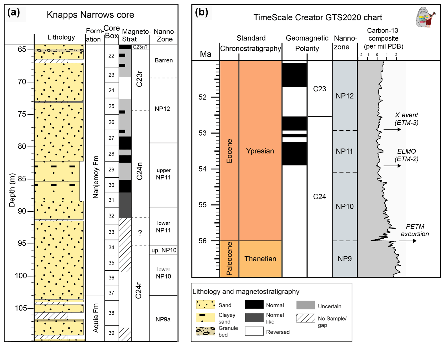
Figure A2(a) The magnetostratigraphy and calcareous nannofossil zones (nanno-zone) of Knapps Narrows core. Note that the C24r C24n reversal boundary was not well determined due to a sampling gap but was well constrained to the interval, where the question mark is placed, based on nannofossils. (b) The latest Paleocene to earliest Eocene timescale from GTS2020 (Gradstein et al., 2020), showing the geomagnetic polarity scale, the calcareous nannofossil zones, and the composite δ13C isotope curve (major δ13C excursions and events are also marked). The excursion of ETM2 aligns with the C24r C24n reversal.
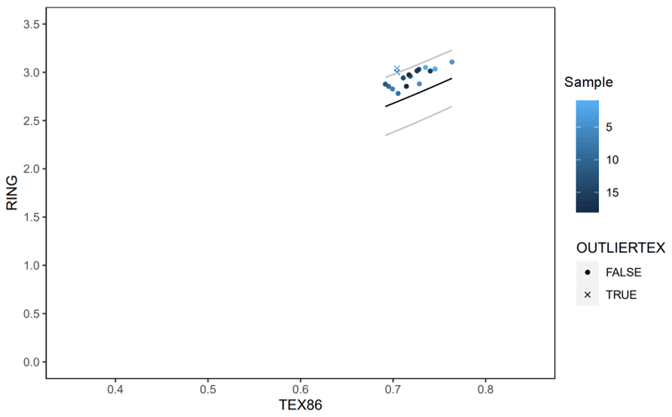
Figure A3Ring index (Zhang et al., 2016) plotted against TEX86 values for Knapps Narrows. Values generally fall within the acceptable range, indicating little non-thermal overprint. The temperature reconstructions obtained from the outliers were in line with independent measurements from δ18O. Moreover, the cutoff for identifying anomalous values is rather conservative (Yi Ge Zhang, written communication, 2022). Therefore, we included these data points in the figures.
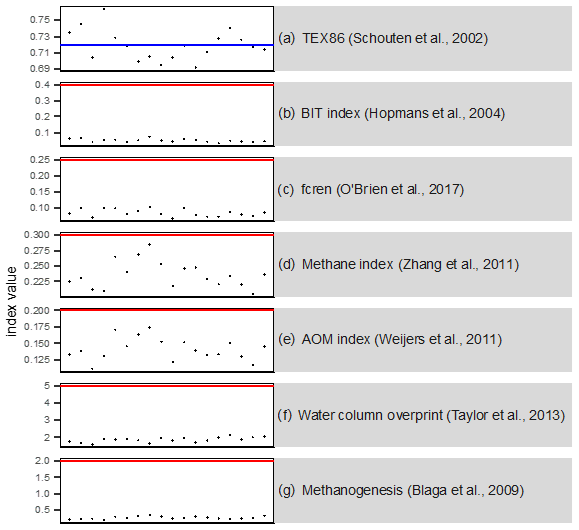
Figure A4Analysis of potential confounding factors for TEX86 paleothermometry for all samples. The red line indicates the cutoff value; red crosses indicate samples exceeding the cutoff (a) TEX86, with the blue line indicating the maximum modern core-top value (∼ 0.72). (b) Low branched and isoprenoid tetraether (BIT) index values indicate the insignificant supply of terrestrial GDGTs. (c) The fractional abundance of crenarchaeol regioisomer relative to total crenarchaeol (fcren) shows no non-thermal contribution of crenarchaeol isomer. (d) Methane index values imply no contribution by methane-metabolizing archaea. (e) The anaerobic oxidation of methane (AOM) ratio values show no contribution by anaerobic methane oxidizers. (f) GDGT2 3 values show no contributions of deep-dwelling archaea. (g) Low GDGT0 cren (crenarchaeol) values show no contribution by methanogenic archaea.
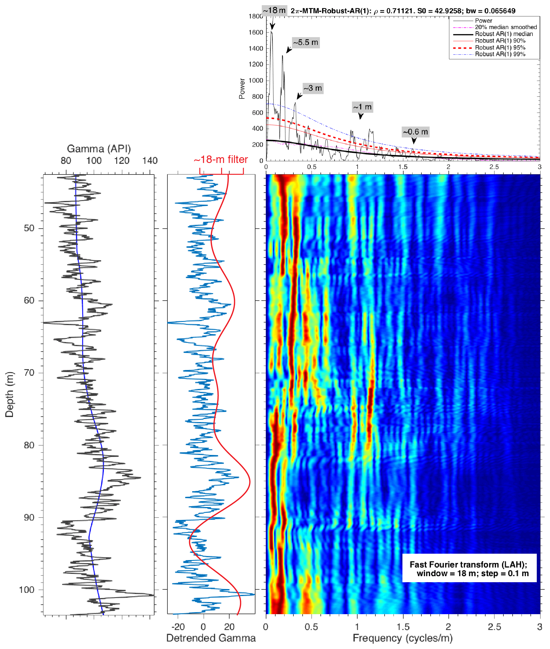
Figure A5Spectral analysis of the detrended gamma data of the Knapps Narrows core (43.5–103.5 m). From left to right are the raw gamma data (solid black line) with the ca. 21 m LOWESS (locally weighted scatterplot smoothing) trend (solid blue line), the detrended gamma data overlain by the ∼ 18 m filter (Gaussian bandwidth at 0.055±0.025), and a spectral analysis of the detrended series. An interpolation of 0.03 m is applied before the spectral analysis. The evolutionary power spectrum (fast Fourier transform; Kodama and Hinnov, 2015) uses an 18 m window. The 2π multi-taper method (MTM) power spectrum shows that the dominant cycles have wavelengths of ∼ 18, ∼ 5.5, 3, ∼ 1, and 0.6 m, respectively.
All data are available via the PANGAEA repository https://doi.org/10.1594/PANGAEA.957710 (Rush et al., 2023).
Samples are available upon request to jstrail@usgs.gov at the Florence Bascom Geoscience Center of the United States Geological Survey.
This paper was prepared by WR, with contributions from all co-authors. Stable isotope measurements, clay mineralogy, carbonate content, age model, and data synthesis were performed by WR. Coring and sampling were performed by JST and MR. Paleomagnetic work and spectral analysis were performed by YZ. Nannofossil biostratigraphy was performed by JST. TEX86 measurements were performed by AS. Palynology was performed by HB. Project oversight and mentoring was provided by JZ.
At least one of the (co-)authors is a member of the editorial board of Climate of the Past. The peer-review process was guided by an independent editor, and the authors also have no other competing interests to declare.
Any use of trade, firm, or product names is for descriptive purposes only and does not imply endorsement by the U.S. Government.
Publisher’s note: Copernicus Publications remains neutral with regard to jurisdictional claims in published maps and institutional affiliations.
Funding for this project has been provided by NSF (grant nos. OCE-1415958, OCE-1658017, and OCE-2103513). We thank Antoinette van den Dikkenberg, Giovanni Dammers, and Natasja Welters (Utrecht University) for analytical and technical assistance. Appy Sluijs thanks the European Research Council for the Consolidator Grant (grant no. 771497; SPANC). Core collection and Marci Robinson have been funded by the USGS Climate Research and Development Program. Jean Self-Trail has been funded by the USGS National Cooperative Geologic Mapping Program. Yang Zhang and the paleomagnetic work have been funded by the Geologic Timescale Foundation.
This research has been supported by the Division of Ocean Sciences (grant nos. OCE-1415958, OCE-1658017, and OCE-2103513) and the H2020 European Research Council (grant no. 771497).
This paper was edited by Luc Beaufort and reviewed by two anonymous referees.
Abels, H. A., Lauretano, V., van Yperen, A. E., Hopman, T., Zachos, J. C., Lourens, L. J., Gingerich, P. D., and Bowen, G. J.: Environmental impact and magnitude of paleosol carbonate carbon isotope excursions marking five early Eocene hyperthermals in the Bighorn Basin, Wyoming, Clim. Past, 12, 1151–1163, https://doi.org/10.5194/cp-12-1151-2016, 2016.
Agnini, C., Fornaciari, E., Raffi, I., Catanzariti, R., Palike, H., Backman, J., and Rio, D.: Biozonation and biochronology of Paleogene calcareous nannofossils from low and middle latitudes, Newsl. Stratigr., 47, 131–181, https://doi.org/10.1127/0078-0421/2014/0042, 2014.
Babila, T. L., Penman, D. E., Standish, C. D., Doubrawa, M., Bralower, T. J., Robinson, M. M., Self-Trail, J. M., Speijer, R. P., Stassen, P., Foster, G. L., and Zachos, J. C.: Surface ocean warming and acidification driven by rapid carbon release precedes Paleocene-Eocene Thermal Maximum, Science Advances, 8, p.eabg1025, https://doi.org/10.1126/sciadv.abg1025, 2022.
Bijl, P. K.: DINOSTRAT: a global database of the stratigraphic and paleolatitudinal distribution of Mesozoic–Cenozoic organic-walled dinoflagellate cysts, Earth Syst. Sci. Data, 14, 579–617, https://doi.org/10.5194/essd-14-579-2022, 2022.
Bijl, P. K., Brinkhuis, H., Egger, L. M., Eldrett, J. S., Frieling, J., Grothe, A., Houben, A. J., Pross, J., Śliwińska, K. K., and Sluijs, A.: Comment on “Wetzeliella and its allies – the `hole' story: a taxonomic revision of the Paleogene dinoflagellate subfamily Wetzelielloideae” by Williams et al. (2015), Palynology, 41, 423–429, https://doi.org/10.1080/01916122.2016.1235056, 2017.
Blair, S. A. and Watkins, D. K.: High-resolution calcareous nannofossil biostratigraphy for the Coniacian/Santonian Stage boundary, Western Interior Basin, Cretaceous Res., 30, 367–384, https://doi.org/10.1016/j.cretres.2008.07.016, 2009.
Blaga, C. I., Reichart, G. J., Heiri, O., and Sinninghe Damsté, J. S.: Tetraether membrane lipid distributions in water-column particulate matter and sediments: a study of 47 European lakes along a north–south transect, J. Paleolimnol., 41, 523–540, https://doi.org/10.1007/s10933-008-9242-2, 2009.
Bowen, G. J., Beerling, D. J., Koch, P. L., Zachos, J. C., and Quattlebaum, T.: A humid climate state during the Palaeocene/Eocene thermal maximum, Nature, 432, 495–499, https://doi.org/10.1038/nature03115, 2004.
Bown, P. and Young, J. R.: Techniques, in: Calcareous Nannofossil Biostratigraphy, edited by: Bown, P. R., Kluwer Academic Press, Cambridge, 16–28, ISBN 0412789701, 1998.
Bralower, T. J., Kump, L. R., Self-Trail, J. M., Robinson, M. M., Lyons, S., Babila, T., Ballaron, E., Freeman, K. H., Hajek, E., Rush, W., and Zachos, J. C.: Evidence for shelf acidification during the onset of the Paleocene-Eocene thermal maximum, Paleoceanography and Paleoclimatology, 33, 1408–1426, https://doi.org/10.1029/2018PA003382, 2018.
Brinkhuis, H., Schouten, S., Collinson, M. E., Sluijs, A., Damsté, J. S. S., Dickens, G. R., Huber, M., Cronin, T. M., Onodera, J., Takahashi, K., and Bujak, J. P.: Episodic fresh surface waters in the Eocene Arctic Ocean, Nature, 441, 606–609, https://doi.org/10.1038/nature04692, 2006.
Carmichael, M. J., Inglis, G. N., Badger, M. P., Naafs, B. D. A., Behrooz, L., Remmelzwaal, S., Monteiro, F. M., Rohrssen, M., Farnsworth, A., Buss, H. L., and Dickson, A. J.: Hydrological and associated biogeochemical consequences of rapid global warming during the Paleocene-Eocene Thermal Maximum, Global Planet. Change, 157, 114–138, https://doi.org/10.1016/j.gloplacha.2017.07.014, 2017.
Chen, Z., Ding, Z., Yang, S., Zhang, C., and Wang, X.: Increased precipitation and weathering across the Paleocene-Eocene Thermal Maximum in central China, Geochem. Geophy. Geosy., 17, 2286–2297, https://doi.org/10.1002/2016GC006333, 2016.
Clechenko, E. R., Kelly, D. C., Harrington, G. J., and Stiles, C. A.: Terrestrial records of a regional weathering profile at the Paleocene-Eocene boundary in the Williston Basin of North Dakota, Geol. Soc. Am. Bull., 119, 428–442, https://doi.org/10.1130/B26010.1, 2007.
Cramer, B. S., Wright, J. D., Kent, D. V., and Aubry, M. P.: Orbital climate forcing of δ13C excursions in the late Paleocene–early Eocene (chrons C24n–C25n), Paleoceanography, 18, 21–25, https://doi.org/10.1029/2003PA000909, 2003.
Cramwinckel, M. J., van der Ploeg, R., Bijl, P. K., Peterse, F., Bohaty, S. M., Röhl, U., Schouten, S., Middelburg, J. J., and Sluijs, A.: Harmful algae and export production collapse in the equatorial Atlantic during the zenith of Middle Eocene Climatic Optimum warmth, Geology, 47, 247–250, https://doi.org/10.1130/G45614.1, 2019.
Crouch, E. M., Dickens, G. R., Brinkhuis, H., Aubry, M.-P., Hollis, C. J., Rogers, K. M., and Visscher, H.: The Apectodinium acme and terrestrial discharge during the Paleocene-Eocene thermal maximum: new palynological, geochemical and calcareous nannoplankton observations at Tawanui, New Zealand, Palaeogeogr. Palaeocl., 194, 387–403, https://doi.org/10.1016/S0031-0182(03)00334-1, 2003.
Darton, N. H.: Structural relations of Cretaceous and Tertiary formations in part of Maryland and Virginia, Geol. Soc. Am. Bull., 62 745–780, https://doi.org/10.1130/0016-7606(1951)62[745:SROCAT]2.0.CO;2, 1951.
Dickens, G. R., Castillo, M. M., and Walker, J. C.: A blast of gas in the latest Paleocene: Simulating first-order effects of massive dissociation of oceanic methane hydrate, Geology, 25, 259–262, https://doi.org/10.1130/0091-7613(1997)025<0259:ABOGIT>2.3.CO;2, 1997.
D'Onofrio, R., Luciani, V., Fornaciari, E., Giusberti, L., Boscolo Galazzo, F., Dallanave, E., Westerhold, T., Sprovieri, M., and Telch, S.: Environmental perturbations at the early Eocene ETM2, H2, and I1 events as inferred by Tethyan calcareous plankton (Terche section, northeastern Italy), Paleoceanography, 31, 1225–1247, https://doi.org/10.1002/2016PA002940, 2016.
Fairbanks, R. G.: The origin of continental shelf and slope water in the New York Bight and Gulf of Maine: evidence from H2 18O H2 16O ratio measurements, J. Geophys. Res.-Oceans, 87, 5796–5808, https://doi.org/10.1029/JC087iC08p05796, 1982.
Dunkley Jones, T., Lunt, D. J., Schmidt, D. N., Ridgwell, A., Sluijs, A., Valdes, P. J., and Maslin, M.: Climate model and proxy data constraints on ocean warming across the Paleocene–Eocene Thermal Maximum, Earth-Sci. Rev., 125, 123–145, https://doi.org/10.1016/j.earscirev.2013.07.004, 2013.
Frieling, J. and Sluijs, A.: Towards quantitative environmental reconstructions from ancient non-analogue microfossil assemblages: Ecological preferences of Paleocene–Eocene dinoflagellates, Earth-Sci. Rev., 185, 956–973, https://doi.org/10.1016/j.earscirev.2018.08.014, 2018.
Frieling, J., Gebhardt, H., Huber, M., Adekeye, O. A., Akande, S. O., Reichart, G.-J., Middelburg, J. J., Schouten, S., and Sluijs, A.: Extreme warmth and heat-stressed plankton in the tropics during the Paleocene-Eocene Thermal Maximum, Science Advances, 3, e1600891, https://doi.org/10.1126/sciadv.1600891, 2017.
Frieling, J., Peterse, F., Lunt, D. J., Bohaty, S. M., Sinninghe Damsté, J. S., Reichart, G. J., and Sluijs, A.: Widespread warming before and elevated barium burial during the Paleocene-Eocene Thermal Maximum: Evidence for methane hydrate release?, Paleoceanography and Paleoclimatology, 34, 546–566, 2019.
Gibson, T. G., Bybell, L. M., and Mason, D. B.: Stratigraphic and climatic implications of clay mineral changes around the Paleocene/Eocene boundary of the northeastern US margin, Sediment. Geol., 134, 65–92, https://doi.org/10.1016/S0037-0738(00)00014-2, 2000.
Gradstein, F. M., Ogg, J. G., Schmitz, M. D., and Ogg, G. M.: Geologic Time Scale 2020, Elsevier, ISBN 978-0-12-824360-2, 2020.
Gutjahr, M., Ridgwell, A., Sexton, P. F., Anagnostou, E., Pearson, P. N., Pälike, H., Norris, R. D., Thomas, E., and Foster, G. L.: Very large release of mostly volcanic carbon during the Palaeocene–Eocene Thermal Maximum, Nature, 548, 573–577, https://doi.org/10.1038/nature23646, 2017.
Harding, I. C., Charles, A. J., Marshall, J. E., Pälike, H., Roberts, A. P., Wilson, P. A., Jarvis, E., Thorne, R., Morris, E., Moremon, R., and Pearce, R. B.: Sea-level and salinity fluctuations during the Paleocene–Eocene thermal maximum in Arctic Spitsbergen, Earth Planet. Sc. Lett., 303, 97–107, https://doi.org/10.1016/j.epsl.2010.12.043, 2011.
Harper, D. T., Zeebe, R., Hönisch, B., Schrader, C. D., Lourens, L. J., and Zachos, J. C.: Subtropical sea-surface warming and increased salinity during Eocene Thermal Maximum 2, Geology, 46, 187–190, https://doi.org/10.1130/G39658.1, 2018.
Harper, D. T., Hönisch, B., Zeebe, R. E., Shaffer, G., Haynes, L. L., Thomas, E., and Zachos, J. C.: The magnitude of surface ocean acidification and carbon release during Eocene Thermal Maximum 2 (ETM-2) and the Paleocene-Eocene Thermal Maximum (PETM), Paleoceanography and Paleoclimatology, 35, e2019PA003699, https://doi.org/10.1029/2019PA003699, 2020.
Ho, S. L. and Laepple, T.: Flat meridional temperature gradient in the early Eocene in the subsurface rather than surface ocean, Nat. Geosci., 9, 606–610, https://doi.org/10.1038/ngeo2763, 2016.
Hollis, C. J., Dunkley Jones, T., Anagnostou, E., Bijl, P. K., Cramwinckel, M. J., Cui, Y., Dickens, G. R., Edgar, K. M., Eley, Y., Evans, D., Foster, G. L., Frieling, J., Inglis, G. N., Kennedy, E. M., Kozdon, R., Lauretano, V., Lear, C. H., Littler, K., Lourens, L., Meckler, A. N., Naafs, B. D. A., Pälike, H., Pancost, R. D., Pearson, P. N., Röhl, U., Royer, D. L., Salzmann, U., Schubert, B. A., Seebeck, H., Sluijs, A., Speijer, R. P., Stassen, P., Tierney, J., Tripati, A., Wade, B., Westerhold, T., Witkowski, C., Zachos, J. C., Zhang, Y. G., Huber, M., and Lunt, D. J.: The DeepMIP contribution to PMIP4: methodologies for selection, compilation and analysis of latest Paleocene and early Eocene climate proxy data, incorporating version 0.1 of the DeepMIP database, Geosci. Model Dev., 12, 3149–3206, https://doi.org/10.5194/gmd-12-3149-2019, 2019.
Hopmans, E. C., Weijers, J. W., Schefuß, E., Herfort, L., Damsté, J. S. S., and Schouten, S.: A novel proxy for terrestrial organic matter in sediments based on branched and isoprenoid tetraether lipids, Earth Planet. Sc. Lett., 224, 107–116, https://doi.org/10.1016/j.epsl.2004.05.012, 2004.
Hurley, S. J., Lipp, J. S., Close, H. G., Hinrichs, K. U., and Pearson, A.: Distribution and export of isoprenoid tetraether lipids in suspended particulate matter from the water column of the Western Atlantic Ocean, Org. Geochem., 116, 90–102, https://doi.org/10.1016/j.orggeochem.2017.11.010, 2018.
Jiang, J., Hu, X., Li, J., BouDagher-Fadel, M., and Garzanti, E.: Discovery of the Paleocene-Eocene Thermal Maximum in shallow-marine sediments of the Xigaze forearc basin, Tibet: A record of enhanced extreme precipitation and siliciclastic sediment flux, Palaeogeogr. Palaeocl., 562, 110095, https://doi.org/10.1016/j.palaeo.2020.110095, 2021.
Jin, S., Kemp, D. B., Jolley, D. W., Vieira, M., Zachos, J. C., Huang, C., Li, M., and Chen, W.: Large-scale, astronomically paced sediment input to the North Sea Basin during the Paleocene Eocene Thermal Maximum, Earth Planet. Sc. Lett., 579, 117340, https://doi.org/10.1016/j.epsl.2021.117340, 2022.
John, C. M., Bohaty, S. M., Zachos, J. C., Sluijs, A., Gibbs, S., Brinkhuis, H., and Bralower, T. J.: North American continental margin records of the Paleocene-Eocene thermal maximum: Implications for global carbon and hydrological cycling, Paleoceanography, 23, PA2217, https://doi.org/10.1029/2007PA001465, 2008.
John, C. M., Banerjee, N. R., Longstaffe, F. J., Sica, C., Law, K. R., and Zachos, J. C.: Clay assemblage and oxygen isotopic constraints on the weathering response to the Paleocene-Eocene thermal maximum, east coast of North America, Geology, 40, 591–594, https://doi.org/10.1130/G32785.1, 2012.
Kemp, S. J., Ellis, M. A., Mounteney, I., and Kender, S.: Palaeoclimatic implications of high-resolution clay mineral assemblages preceding and across the onset of the Palaeocene–Eocene Thermal Maximum, North Sea Basin, Clay Miner., 51, 793–813, https://doi.org/10.1180/claymin.2016.051.5.08, 2016.
Kodama, K. P. and Hinnov, L.: Rock Magnetic Cyclostratigraphy, John Wiley and Sons, 5, 165, https://doi.org/10.1002/9781118561294, 2015.
Kiehl, J. T., Shields, C. A., Snyder, M. A., Zachos, J. C., and Rothstein, M.: Greenhouse-and orbital-forced climate extremes during the early Eocene, Philos. T. R. Soc. A, 376, 20170085, https://doi.org/10.1098/rsta.2017.0085, 2018.
Kim, J. H., Van der Meer, J., Schouten, S., Helmke, P., Willmott, V., Sangiorgi, F., Koç, N., Hopmans, E. C., and Damsté, J. S. S.: New indices and calibrations derived from the distribution of crenarchaeal isoprenoid tetraether lipids: Implications for past sea surface temperature reconstructions, Geochim. Cosmochim. Ac., 74, 4639–4654, https://doi.org/10.1016/j.gca.2010.05.027, 2010.
Kopp, R. E., Schumann, D., Raub, T. D., Powars, D. S., Godfrey, L. V., Swanson-Hysell, N. L., Maloof, A. C., and Vali, H.: Appalachian Amazon? Magnetofossil evidence for the development of a tropical river-like system in the mid-Atlantic United States during the Paleocene-Eocene thermal maximum, Paleoceanography, 24, PA4211, https://doi.org/10.1029/2009PA001783, 2009.
Krishnan, S., Pagani, M., Huber, M., and Sluijs, A.: High latitude hydrological changes during the Eocene Thermal Maximum 2, Earth Planet. Sc. Lett., 404, 167–177, https://doi.org/10.1016/j.epsl.2014.07.029, 2014.
Lauretano, V., Littler, K., Polling, M., Zachos, J. C., and Lourens, L. J.: Frequency, magnitude and character of hyperthermal events at the onset of the Early Eocene Climatic Optimum, Clim. Past, 11, 1313–1324, https://doi.org/10.5194/cp-11-1313-2015, 2015.
Li, M. S., Kump, L., Hinnov, L. A., and Mann, M.: Tracking variable sedimentation rates and astronomical forcing in Phanerozoic paleoclimate proxy series with evolutionary correlation coefficients and hypothesis testing, Earth Planet. Sc. Lett., 501, 165–179, https://doi.org/10.1016/j.epsl.2018.08.041, 2018.
Li, M. S., Hinnov, L., and Kump, L.: Acycle: Time-series analysis software for paleoclimate projects and education, Comput. Geosci., 127, 12–22, https://doi.org/10.1016/j.cageo.2019.02.011, 2019.
Li, M. S., Bralower, T. J., Kump, L. R., Self-Trail, J. M., Zachos, J. C., Rush, W. D., and Robinson, M. M.: Astrochronology of the Paleocene-Eocene Thermal Maximum on the Atlantic Coastal Plain, Nat. Commun., 13, 5618, https://doi.org/10.1038/s41467-022-33390-x, 2022.
Littler, K., Röhl, U., Westerhold, T., and Zachos, J. C.: A high-resolution benthic stable-isotope record for the South Atlantic: Implications for orbital-scale changes in Late Paleocene–Early Eocene climate and carbon cycling, Earth Planet. Sc. Lett., 401, 18–30, https://doi.org/10.1016/j.epsl.2014.05.054, 2014.
Lourens, L. J., Sluijs, A., Kroon, D., Zachos, J. C., Thomas, E., Röhl, U., Bowles, J., and Raffi, I.: Astronomical pacing of late Palaeocene to early Eocene global warming events, Nature, 435, 1083–1087, https://doi.org/10.1038/nature03814, 2005.
Marchitto, T. M., Curry, W. B., Lynch-Stieglitz, J., Bryan, S. P., Cobb, K. M., and Lund, D. C.: Improved oxygen isotope temperature calibrations for cosmopolitan benthic foraminifera, Geochim. Cosmochim. Ac., 130, 1–11, https://doi.org/10.1016/j.gca.2013.12.034, 2014.
Lyons, S. L., Baczynski, A. A., Babila, T. L., Bralower, T. J., Hajek, E. A., Kump, L. R., Polites, E. G., Self-Trail, J. M., Trampush, S. M., Vornlocher, J. R., and Zachos, J. C.: Palaeocene–Eocene thermal maximum prolonged by fossil carbon oxidation, Nat. Geosci., 12, 54–60, https://doi.org/10.1038/s41561-018-0277-3, 2019.
Martini, W.: Standard Tertiary and Quaternary calcareous nannoplankton zonation, in: Proceedings of the 2nd Planktonic Conference, Roma, edited by: Farinacci, A., 2, 739–785, 1971.
Nicolo, M. J., Dickens, G. R., Hollis, C. J., and Zachos, J. C.: Multiple early Eocene hyperthermals: Their sedimentary expression on the New Zealand continental margin and in the deep sea, Geology, 35, 699–702, https://doi.org/10.1130/G23648A.1, 2007.
O'Brien, C. L., Robinson, S. A., Pancost, R. D., Damsté, J. S. S., Schouten, S., Lunt, D. J., Alsenz, H., Bornemann, A., Bottini, C., Brassell, S. C., and Farnsworth, A.: Cretaceous sea-surface temperature evolution: Constraints from TEX86 and planktonic foraminiferal oxygen isotopes, Earth-Sci. Rev., 172, 224–247, https://doi.org/10.1016/j.earscirev.2017.07.012, 2017.
Pagani, M., Pedentchouk, N., Huber, M., Sluijs, A., Schouten, S., Brinkhuis, H., Sinninghe Damsté, J. S., and Dickens, G. R.: Arctic hydrology during global warming at the Palaeocene/Eocene thermal maximum, Nature, 442, 671–675, https://doi.org/10.1038/nature05043, 2006.
Penman, D. E., Hönisch, B., Zeebe, R. E., Thomas, E., and Zachos, J. C.: Rapid and sustained surface ocean acidification during the Paleocene-Eocene Thermal Maximum, Paleoceanography, 29, 357–369, https://doi.org/10.1002/2014PA002621, 2014.
Pfahl, S., O'Gorman, P. A., and Fischer, E. M.: Understanding the regional pattern of projected future changes in extreme precipitation, Nat. Clim. Chang., 7, 423–427, https://doi.org/10.1038/nclimate3287, 2017.
Pogge von Strandmann, P. A., Jones, M. T., West, A. J., Murphy, M. J., Stokke, E. W., Tarbuck, G., Wilson, D. J., Pearce, C. R., and Schmidt, D. N.: Lithium isotope evidence for enhanced weathering and erosion during the Paleocene-Eocene Thermal Maximum, Science Advances, 7, p.eabh4224, https://doi.org/10.1126/sciadv.abh4224, 2021.
Poppe, L. J., Paskevich, V. F., Hathaway, J. C., and Blackwood, D. S.: A laboratory manual for X-ray powder diffraction, US Geological Survey open-file report, 1, 1–88, https://doi.org/10.3133/ofr0141, 2001.
Przybylski, P. A., Ogg, J. G., Wierzbowski, A., Coe, A. L., Hounslow, M. W., Wright, J. K., Atrops, F., and Settles, E.: Magnetostratigraphic correlation of the Oxfordian–Kimmeridgian boundary, Earth Planet. Sc. Lett., 289, 256–272, https://doi.org/10.1016/j.epsl.2009.11.014, 2010.
Ramos, E. J., Breecker, D. O., Barnes, J. D., Li, F., Gingerich, P. D., Loewy, S. L., Satkoski, A. M., Baczynski, A. A., Wing, S. L., Miller, N. R., and Lassiter, J. C.: Swift Weathering Response on Floodplains During the Paleocene-Eocene Thermal Maximum, Geophys. Res. Lett., 49, p.e2021GL097436, https://doi.org/10.1029/2021GL097436, 2022.
Reichart, G.-J. and Brinkhuis, H.: Late Quaternary Protoperidinium cysts as indicators of paleoproductivity in the northern Arabian Sea, Mar. Micropaleontol., 49, 303–315, https://doi.org/10.1016/S0377-8398(03)00050-1, 2003.
Reinhardt, L., von Gosen, W., Lückge, A., Blumenberg, M., Galloway, J. M., West, C. K., Sudermann, M., and Dolezych, M.: Geochemical indications for the Paleocene-Eocene Thermal Maximum (PETM) and Eocene Thermal Maximum 2 (ETM-2) hyperthermals in terrestrial sediments of the Canadian Arctic, Geosphere, 18, 327–349, https://doi.org/10.1130/GES02398.1, 2022.
Reynolds, P., Planke, S., Millett, J. M., Jerram, D. A., Trulsvik, M., Schofield, N., and Myklebust, R.: Hydrothermal vent complexes offshore Northeast Greenland: A potential role in driving the PETM, Earth Planet. Sc. Lett., 467, 72–78, https://doi.org/10.1016/j.epsl.2017.03.031, 2017.
Richaud, B., Kwon, Y. O., Joyce, T. M., Fratantoni, P. S., and Lentz, S. J.: Surface and bottom temperature and salinity climatology along the continental shelf off the Canadian and US East Coasts, Cont. Shelf Res., 124, 165–181, https://doi.org/10.1016/j.csr.2016.06.005, 2016.
Robert, C. and Kennett, J. P.: Antarctic subtropical humid episode at the Paleocene-Eocene boundary: Clay-mineral evidence, Geology, 22, 211–214, https://doi.org/10.1130/0091-7613(1994)022<0211:ASHEAT>2.3.CO;2, 1994.
Rush, W. D., Kiehl, J. T., Shields, C. A., and Zachos, J. C.: Increased frequency of extreme precipitation events in the North Atlantic during the PETM: Observations and theory, Palaeogeogr. Palaeocl., 568, 110289, https://doi.org/10.1016/j.palaeo.2021.110289, 2021.
Rush, W., Self-Trail, J., Zhang, Y., Sluijs, A., Brinkhuis, H., Zachos, J. C., Ogg, J. G., and Robinson, M. M.: Knapps Narrows Calcareous Nannofossil Biozonation over ETM2 and H2, PANGAEA [data set], https://doi.org/10.1594/PANGAEA.957710, 2023.
Sabat, M. A.: Gravity anomalies associated with the Salisbury embayment, Maryland–southern Delaware, Geology, 5, 433-436, https://doi.org/10.1130/0091-7613(1977)5<433:GAAWTS>2.0.CO;2, 1977.
Schmitz, B. and Pujalte, V.: Abrupt increase in seasonal extreme precipitation at the Paleocene-Eocene boundary, Geology, 35, 215–218, https://doi.org/10.1130/G23261A.1, 2007.
Schouten, S., Hopmans, E. C., Schefuß, E., and Sinninghe Damsté, J. S.: Distributional variations in marine crenarchaeotal membrane lipids: a new tool for reconstructing ancient sea water temperatures?, Earth Planet. Sc. Lett., 204, 265–274, https://doi.org/10.1016/S0012-821X(02)00979-2, 2002.
Scotese, C.: Atlas of Paleogene Paleogeographic maps, Maps 8-15, Volume 1, The Cenozoic, PALEOMAP Atlas for ArcGIS, Mollweide Projection, PALEOMAP Project, Evanston, IL, https://doi.org/10.13140/2.1.3417.6961, 2014.
Singer, A.: The paleoclimatic interpretation of clay minerals in soils and weathering profiles, Earth-Sci. Rev., 15, 303–326, https://doi.org/10.1016/0012-8252(80)90113-0, 1980.
Self-Trail, J. M., Powars, D. S., Watkins, D. K., and Wandless, G. A.: Calcareous nannofossil assemblage changes across the Paleocene–Eocene Thermal Maximum: Evidence from a shelf setting, Mar. Micropaleontol., 92, 61–80, https://doi.org/10.1016/j.marmicro.2012.05.003, 2012.
Self-Trail, J. M., Powars, D. S., Zhang, Y., Ogg, J. G., and Fung, M. K.: A very (very) preliminary chronostratigraphic framework of an expanded and structurally controlled early Eocene section from the Knapps Narrows core, Salisbury Embayment, USA, CBEP 2017, UT, 3–8 September, p. 121, 2017a.
Self-Trail, J. M., Robinson, M. M., Bralower, T. J., Sessa, J. A., Hajek, E. A., Kump, L. R., Trampush, S. M., Willard, D. A., Edwards, L. E., Powars, D. S., and Wandless, G. A.: Shallow marine response to global climate change during the Paleocene-Eocene Thermal Maximum, Salisbury Embayment, USA, Paleoceanography, 32, 710–728, https://doi.org/10.1002/2017PA003096, 2017b.
Slotnick, B. S., Dickens, G. R., Nicolo, M. J., Hollis, C. J., Crampton, J. S., Zachos, J. C., and Sluijs, A.: Large-amplitude variations in carbon cycling and terrestrial weathering during the latest Paleocene and earliest Eocene: The record at Mead Stream, New Zealand, J. Geol., 120, 487–505, https://doi.org/10.1086/666743, 2012.
Sluijs, A. and Brinkhuis, H.: A dynamic climate and ecosystem state during the Paleocene-Eocene Thermal Maximum: inferences from dinoflagellate cyst assemblages on the New Jersey Shelf, Biogeosciences, 6, 1755–1781, https://doi.org/10.5194/bg-6-1755-2009, 2009.
Sluijs, A. and Dickens, G. R.: Assessing offsets between the δ13C of sedimentary components and the global exogenic carbon pool across early Paleogene carbon cycle perturbations, Global Biogeochem. Cy., 26, GB4005, https://doi.org/10.1029/2011GB004224, 2012.
Sluijs, A., Pross, J., and Brinkhuis, H.: From greenhouse to icehouse; organic-walled dinoflagellate cysts as paleoenvironmental indicators in the Paleogene, Earth-Sci. Rev., 68, 281–315, https://doi.org/10.1016/j.earscirev.2004.06.001, 2005.
Sluijs, A., Brinkhuis, H., Schouten, S., Bohaty, S. M., John, C. M., Zachos, J. C., Reichart, G. J., Sinninghe Damsté, J. S., Crouch, E. M., and Dickens, G. R.: Environmental precursors to rapid light carbon injection at the Palaeocene/Eocene boundary, Nature, 450, 1218–1221, https://doi.org/10.1038/nature06400, 2007.
Sluijs, A., Schouten, S., Donders, T. H., Schoon, P. L., Röhl, U., Reichart, G. J., Sangiorgi, F., Kim, J. H., Sinninghe Damsté, J. S., and Brinkhuis, H.: Warm and wet conditions in the Arctic region during Eocene Thermal Maximum 2, Nat. Geosci., 2, 777–780, https://doi.org/10.1038/ngeo668, 2009.
Sluijs, A., van Roij, L., Harrington, G. J., Schouten, S., Sessa, J. A., LeVay, L. J., Reichart, G.-J., and Slomp, C. P.: Warming, euxinia and sea level rise during the Paleocene–Eocene Thermal Maximum on the Gulf Coastal Plain: implications for ocean oxygenation and nutrient cycling, Clim. Past, 10, 1421–1439, https://doi.org/10.5194/cp-10-1421-2014, 2014.
Sluijs, A., van Roij, L., Frieling, J., Laks, J., and Reichart, G. J.: Single-species dinoflagellate cyst carbon isotope ecology across the Paleocene-Eocene Thermal Maximum, Geology, 46, 79–82, https://doi.org/10.1130/G39598.1, 2018.
Sluijs, A., Frieling, J., Inglis, G. N., Nierop, K. G. J., Peterse, F., Sangiorgi, F., and Schouten, S.: Late Paleocene–early Eocene Arctic Ocean sea surface temperatures: reassessing biomarker paleothermometry at Lomonosov Ridge, Clim. Past, 16, 2381–2400, https://doi.org/10.5194/cp-16-2381-2020, 2020.
Speijer, R. P., Pälike, H., Hollis, C. J., Hooker, J. J., and Ogg, J. G.: Chapter 28 – The Paleogene Period, edited by: Gradstein, F. M., Ogg, J. G., Schmitz, M. D., and Ogg, G. M., Geologic Time Scale 2020, Elsevier, 1087–1140, ISBN 9780128243602, https://doi.org/10.1016/B978-0-12-824360-2.00028-0, 2020.
Stap, L., Lourens, L. J., Thomas, E., Sluijs, A., Bohaty, S., and Zachos, J. C.: High-resolution deep-sea carbon and oxygen isotope records of Eocene Thermal Maximum 2 and H2, Geology, 38, 607–610, https://doi.org/10.1130/G30777.1, 2010.
Stassen, P., Thomas, E., and Speijer, R. P.: Integrated stratigraphy of the Paleocene-Eocene thermal maximum in the New Jersey Coastal Plain: Toward understanding the effects of global warming in a shelf environment, Paleoceanography, 27, PA4210, https://doi.org/10.1029/2012PA002323, 2012a.
Stassen, P., Steurbaut, E., Morsi, A. M., Schulte, P., and Speijer, R.: Biotic impact of Eocene Thermal Maximum 2 in a shelf setting (Dababiya, Egypt). Austrian J. Earth Sci., 105, 154–160, 2012b.
Swain, D. L., Langenbrunner, B., Neelin, J. D., and Hall, A.: Increasing precipitation volatility in twenty-first-century California, Nat. Clim. Chang., 8, 427–433, https://doi.org/10.1038/s41558-018-0140-y, 2018.
Taylor, K. W., Huber, M., Hollis, C. J., Hernandez-Sanchez, M. T., and Pancost, R. D.: Re-evaluating modern and Palaeogene GDGT distributions: Implications for SST reconstructions, Global Planet. Change, 108, 158–174, https://doi.org/10.1016/j.gloplacha.2013.06.011, 2013.
Thomas, E. and Zachos, J. C.: Was the late Paleocene thermal maximum a unique event?, Gff, 122, 169–170, https://doi.org/10.1080/11035890001221169, 2000.
Tipple, B. J., Pagani, M., Krishnan, S., Dirghangi, S. S., Galeotti, S., Agnini, C., Giusberti, L., and Rio, D.: Coupled high-resolution marine and terrestrial records of carbon and hydrologic cycles variations during the Paleocene–Eocene Thermal Maximum (PETM), Earth Planet. Sc. Lett., 311, 82–92, https://doi.org/10.1016/j.epsl.2011.08.045, 2011.
Trampush, S. M. and Hajek, E. A.: Preserving proxy records in dynamic landscapes: Modeling and examples from the Paleocene-Eocene Thermal Maximum, Geology, 45, 967–970, https://doi.org/10.1130/G39367.1, 2017.
van der Weijst, C. M. H., van der Laan, K. J., Peterse, F., Reichart, G.-J., Sangiorgi, F., Schouten, S., Veenstra, T. J. T., and Sluijs, A.: A 15-million-year surface- and subsurface-integrated TEX86 temperature record from the eastern equatorial Atlantic, Clim. Past, 18, 1947–1962, https://doi.org/10.5194/cp-18-1947-2022, 2022.
van Hinsbergen, D. J. J., de Groot, L. V., van Schaik, S. J., Spakman, W., Bijl, P. K., Sluijs, A., Langereis, C. G., and Brinkhuis, H.: A Paleolatitude Calculator for Paleoclimate Studies, PLOS ONE, 10, e0126946, https://doi.org/10.1371/journal.pone.0126946, 2015.
Vervoort, P., Kirtland Turner, S., Rochholz, F., and Ridgwell, A.: Earth System Model Analysis of How Astronomical Forcing Is Imprinted Onto the Marine Geological Record: The Role of the Inorganic (Carbonate) Carbon Cycle and Feedbacks, Paleoceanography and Paleoclimatology, 36, e2020PA004090, https://doi.org/10.1029/2020PA004090, 2021.
Weijers, J. W., Lim, K. L., Aquilina, A., Sinninghe Damsté, J. S., and Pancost, R. D.: Biogeochemical controls on glycerol dialkyl glycerol tetraether lipid distributions in sediments characterized by diffusive methane flux. Geochem. Geophy. Geosy., 12, Q10010, https://doi.org/10.1029/2011GC003724, 2011.
Westerhold, T., Röhl, U., Laskar, J., Raffi, I., Bowles, J., Lourens, L. J., and Zachos, J. C.: On the duration of magnetochrons C24r and C25n and the timing of early Eocene global warming events: Implications from the Ocean Drilling Program Leg 208 Walvis Ridge depth transect, Paleoceanography, 22, PA2201, https://doi.org/10.1029/2006PA001322, 2007.
Westerhold, T., Röhl, U., Wilkens, R. H., Gingerich, P. D., Clyde, W. C., Wing, S. L., Bowen, G. J., and Kraus, M. J.: Synchronizing early Eocene deep-sea and continental records – cyclostratigraphic age models for the Bighorn Basin Coring Project drill cores, Clim. Past, 14, 303–319, https://doi.org/10.5194/cp-14-303-2018, 2018.
Willard, D. A., Donders, T. H., Reichgelt, T., Greenwood, D. R., Sangiorgi, F., Peterse, F., Nierop, K. G., Frieling, J., Schouten, S., and Sluijs, A.: Arctic vegetation, temperature, and hydrology during Early Eocene transient global warming events, Global Planet. Change, 178, 139–152, https://doi.org/10.1016/j.gloplacha.2019.04.012, 2019.
Williams, G. L., Brinkhuis, H., Pearce, M. A., Fensome, R. A., and Weegink, J. W.: Southern Ocean and global dinoflagellate cyst events compared: index events for the Late Cretaceous–Neogene, in: Proc. ODP, Sci. Results, 189, edited by: Exon, N. F., Kennett, J. P., and Malone, M. J., College Station, TX (Ocean Drilling Program), 1–98, https://doi.org/10.2973/odp.proc.sr.189.107, 2004.
Williams, G. L., Damassa, S. P., Fensome, R. A., and Guerstein, G. R.: A response to “Comment to Wetzeliella and its allies – the `hole' story: a taxonomic revision of the Paleogene dinoflagellate subfamily Wetzelielloideae by Williams et al.(2015)”, Palynology, 41, 430–437, https://doi.org/10.1080/01916122.2017.1283367, 2017.
Zachos, J. C., Röhl, U., Schellenberg, S. A., Sluijs, A., Hodell, D. A., Kelly, D. C., Thomas, E., Nicolo, M., Raffi, I., Lourens, L. J., and McCarren, H.: Rapid acidification of the ocean during the Paleocene-Eocene thermal maximum, Science, 308, 1611–1615, https://doi.org/10.1126/science.1109004, 2005.
Zachos, J. C., Schouten, S., Bohaty, S., Quattlebaum, T., Sluijs, A., Brinkhuis, H., Gibbs, S. J., and Bralower, T. J.: Extreme warming of mid-latitude coastal ocean during the Paleocene-Eocene Thermal Maximum: Inferences from TEX86 and isotope data, Geology, 34, 737–740, https://doi.org/10.1130/G22522.1, 2006.
Zachos, J. C., Dickens, G. R., and Zeebe, R. E.: An early Cenozoic perspective on greenhouse warming and carbon-cycle dynamics, Nature, 451, 279–283, https://doi.org/10.1038/nature06588, 2008.
Zachos, J. C., McCarren, H., Murphy, B., Röhl, U., and Westerhold, T.: Tempo and scale of late Paleocene and early Eocene carbon isotope cycles: Implications for the origin of hyperthermals, Earth Planet. Sc. Lett., 299, 242–249, 2010.
Zeebe, R. E. and Lourens, L. J.: Solar System chaos and the Paleocene–Eocene boundary age constrained by geology and astronomy, Science, 365, 926–929, https://doi.org/10.1126/science.aax0612, 2019.
Zeebe, R. E., Westerhold, T., Littler, K., and Zachos, J. C.: Orbital forcing of the Paleocene and Eocene carbon cycle, Paleoceanography, 32, 440–465, https://doi.org/10.1002/2016PA003054, 2017.
Zhang, C. and Ogg, J. G.: An integrated paleomagnetic analysis program for stratigraphy labs and research projects. Comput. Geosci., 29, 613–625, https://doi.org/10.1016/S0098-3004(03)00034-7, 2003.
Zhang, Y. G., Zhang, C. L., Liu, X. L., Li, L., Hinrichs, K. U., and Noakes, J. E.: Methane Index: A tetraether archaeal lipid biomarker indicator for detecting the instability of marine gas hydrates, Earth Planet. Sc. Lett., 307, 525–534, https://doi.org/10.1016/j.epsl.2011.05.031, 2011.
Zhang, Y. G., Pagani, M., and Wang, Z.: Ring Index: A new strategy to evaluate the integrity of TEX86 paleothermometry, Paleoceanography, 31, 220–232, 2016.
Zonneveld, K. A., Marret, F., Versteegh, G. J., Bogus, K., Bonnet, S., Bouimetarhan, I., Crouch, E., de Vernal, A., Elshanawany, R., Edwards, L., and Esper, O.: Atlas of modern dinoflagellate cyst distribution based on 2405 data points, Rev. Palaeobot. Palyno., 191, 1–197, https://doi.org/10.1016/j.revpalbo.2012.08.003, 2013.