


ABSTRACT
The Interstellar Boundary Explorer (IBEX) observes the IBEX ribbon, which stretches across much of the sky observed in energetic neutral atoms (ENAs). The ribbon covers a narrow (∼20°–50°) region that is believed to be roughly perpendicular to the interstellar magnetic field. Superimposed on the IBEX ribbon is the globally distributed flux that is controlled by the processes and properties of the heliosheath. This is a second study that utilizes a previously developed technique to separate ENA emissions in the ribbon from the globally distributed flux. A transparency mask is applied over the ribbon and regions of high emissions. We then solve for the globally distributed flux using an interpolation scheme. Previously, ribbon separation techniques were applied to the first year of IBEX-Hi data at and above 0.71 keV. Here we extend the separation analysis down to 0.2 keV and to five years of IBEX data enabling first maps of the ribbon and the globally distributed flux across the full sky of ENA emissions. Our analysis shows the broadening of the ribbon peak at energies below 0.71 keV and demonstrates the apparent deformation of the ribbon in the nose and heliotail. We show global asymmetries of the heliosheath, including both deflection of the heliotail and differing widths of the lobes, in context of the direction, draping, and compression of the heliospheric magnetic field. We discuss implications of the ribbon maps for the wide array of concepts that attempt to explain the ribbon's origin. Thus, we present the five-year separation of the IBEX ribbon from the globally distributed flux in preparation for a formal IBEX data release of ribbon and globally distributed flux maps to the heliophysics community.
Export citation and abstract BibTeX RIS
1. INTRODUCTION
The Interstellar Boundary Explorer (IBEX) mission has two sensors, IBEX-Lo (Fuselier et al. 2009b) and IBEX-Hi (Funsten et al. 2009a) that measure energetic neutral atoms (ENAs) with energies of ∼10 eV to 2 keV and ∼300 eV to 6 keV, respectively (McComas et al. 2009a, 2009b). The global ENA maps from IBEX characterize the interactions of the solar wind with the local interstellar medium. The first global maps of the heliosphere in ENAs (McComas et al. 2009a; Schwadron et al. 2009a; Fuselier et al. 2009a; Funsten et al. 2009b) showed the presence of a narrow ribbon (∼20°–40° wide) of elevated emissions that forms a circular arc roughly centered on ecliptic coordinates (long., lat.) ∼(219 2 ± 13, 399 ± 23; Funsten et al. 2013). Comparisons between models of the outer heliosheath and the ribbon suggested that LISM magnetic field in the outer heliosheath is roughly perpendicular to the IBEX ribbon (or where B · r = 0, where r is the radial line-of-sight (LOS) and B is the interstellar magnetic field, McComas et al. 2009a; Schwadron et al. 2009a; Ratkiewicz et al. 2012). The center of the ribbon can potentially be considered as a proxy for the direction of the local interstellar magnetic field direction (Grygorczuk et al. 2011). The ribbon center direction is within ∼33° ± 20° of the magnetic field direction derived from interstellar polarization data using stars within 40 pc (Frisch et al. 2012; Frisch & Schwadron 2013). Recently, (Schwadron et al. 2014) showed that the anisotropy maps of high-energy (TeV) cosmic rays provide independent confirmation of the interstellar magnetic field orientation inferred from the IBEX ribbon center. Therefore, mounting evidence shows that the center of the ribbon is the direction of interstellar magnetic field in the outer heliosheath.
The ribbon flux is notably superimposed on a slowly varying ENA flux that is referred to as the globally distributed flux (GDF) and is likely a separate emission population. The purpose of this paper is to utilize a method previously developed (Schwadron et al. 2011) to separate the GDF from the ribbon and discuss the properties of the two ENA populations. The first separation of the IBEX ribbon from the GDF was performed using the first year of IBEX-Hi data for the energy range from 0.7 to 4.3 keV. This study builds on (Schwadron et al. 2011) by performing ribbon separation using the first five years of IBEX-Hi and IBEX-Lo data covering a broadened energy range from 0.2 to 4.3 keV.
The GDF exhibits broad angular distributions far more consistent with original predictions of ENA maps from models (Prested et al. 2008; Schwadron et al. 2009a, 2009b). This led to the suggestion that the GDF most likely forms from charge exchange between interstellar neutrals and plasma in the inner heliosheath (McComas et al. 2009a; Schwadron et al. 2009a, 2011; Fuselier et al. 2009a; Funsten et al. 2009b). Therefore, maps of GDF are used to study properties of the inner heliosheath (Livadiotis et al. 2012). Maps of the IBEX ribbon are often used to test models of ribbon formation (see McComas et al. 2010, 2014b; Schwadron et al. 2011), to test the properties of the interstellar cloud surrounding the heliosphere (Frisch et al. 2010; Heerikhuisen et al. 2010, 2014; Ratkiewicz et al. 2012; Schwadron et al. 2014), and in comparison with observations of the interstellar magnetic field (e.g., Frisch et al. 2012; Frisch & Schwadron 2013). The maps of the GDF and the ribbon provided here will be released as new data products to the heliophysics community, allowing comparison between results of IBEX and models for both the ribbon and the inner heliosheath.
2. SEPARATION OF THE RIBBON FROM GLOBALLY DISTRIBUTED FLUX FROM THE COMBINED FIVE YEARS OF OBSERVATIONS
The starting point for our analysis is a set of global maps that are a statistically weighted combination of the first five years ENA sky maps (McComas et al. 2014a), shown in Figure 1. These maps are Compton–Getting corrected to the central energy of the sensor at every energy step in the inertial reference frame at 1 AU. Survival probability corrections are also applied. Therefore, the maps represent incident ENA fluxes from ∼100 AU (i.e., the outer heliosphere). The ENA maps are formed from data taken only when the sensors view the heliosphere in the ram direction (with a positive prograde component). For this "ram viewing," the Compton–Getting correction acts to suppress noise in the ENA fluxes (McComas et al. 2012). All maps have also been filtered according to signal-to-noise (S/N, ratio of flux to the standard deviation) such that any pixel with S/N <3 is zeroed.
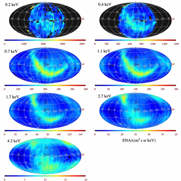
Figure 1. Our analysis begins with survival probability and Comptom–Getting corrected flux maps from the IBEX-Lo and IBEX-Hi ENA imagers over the first 5 years of the mission (McComas et al. 2014a). Note that the color coding scale varies by a factor of 20 between the individual panels.
Download figure:
Standard image High-resolution imageThe maps in Figure 1 include the Compton–Getting and survival probability corrected IBEX-Lo ENA fluxes at 0.2 and 0.4 keV, also including only ram viewing. The IBEX-Lo maps are incomplete covering only the region from −30° to −180° in ecliptic longitude as the result of including only ram viewing and excluding time periods of high background when IBEX moves through the terrestrial magnetosphere.
IBEX-Lo maps have been corrected by subtraction of the sputtering contributions from O and H, as detailed in the Appendix of (McComas et al. 2014a). The sputtering factors have been calculated using a combination of calibration and flight data. We also include corrections to IBEX-Lo geometric factors due to changes in the IBEX-Lo post acceleration (PAC) voltage and changes in data throughput from the instrument to the central electronics unit (throughput is defined as the percentage of measured events that survive in the data stream to the central electronics unit). The average throughput was 80% in IBEX-Lo ESA 5, 94% in IBEX-Lo ESA 6, and 96% in ESA 7 and 8 prior to orbit 168. After orbit 168, the throughput was improved to ∼100% by removing unused housekeeping in the data stream. In addition, the PAC voltage was lowered in orbit 177 to exclude backgrounds, which required subsequent adjustment to the IBEX-Lo geometric factors. Finally, the IBEX-Lo ESA 5 subtracts a small background rate of 0.005 ± 0.001 s−1 (A. Galli et al. 2014, in preparation; there is no background correction applied for IBEX-Lo ESA 6). Background rates are also subtracted from IBEX-Hi data, as detailed by (McComas et al. 2014a).
We have applied the same techniques as detailed in (Schwadron et al. 2011) to separate the ribbon from the GDF. The technique proceeds by first rotating the global maps of IBEX into a frame with a polar axis near the ribbon center, taking advantage of the ribbon circularity (eccentricity ∼0.3, Funsten et al. 2013). This rotation makes it relatively straightforward to perform fits to the ribbon and then use these fits to separate out the ribbon from the GDF ENA populations. The separation technique is entirely independent at different energy steps. The method of ribbon separation is not strongly dependent on the choice of ribbon center. For convenience, we have adopted a ribbon center at ecliptic longitude 221° and ecliptic latitude 39°, which is within 2° from the ribbon center derived by (Funsten et al. 2013). Figures 2–4 show the separated ribbon flux maps and Figures 5–7 shows the GDF maps in ecliptic, equatorial, and galactic coordinates.
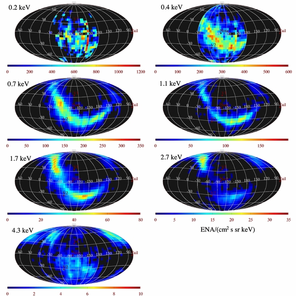
Figure 2. IBEX ribbon separated from the GDF in ecliptic coordinates using the first 5 years of IBEX data.
Download figure:
Standard image High-resolution image
Figure 3. IBEX ribbon separated from the GDF in equatorial coordinates using the first 5 years of IBEX data.
Download figure:
Standard image High-resolution image
Figure 4. IBEX ribbon separated from the GDF in galactic coordinates using the first 5 years of IBEX data.
Download figure:
Standard image High-resolution image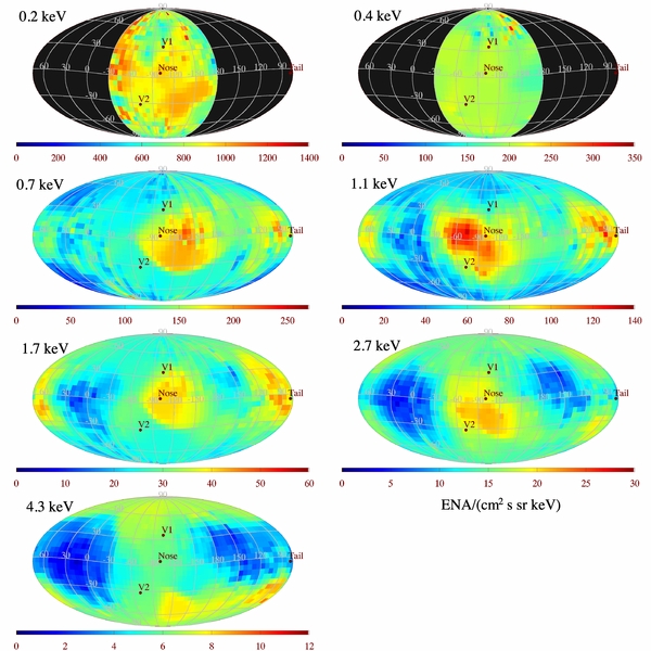
Figure 5. GDF in ecliptic coordinates using the first 5 years of IBEX data.
Download figure:
Standard image High-resolution image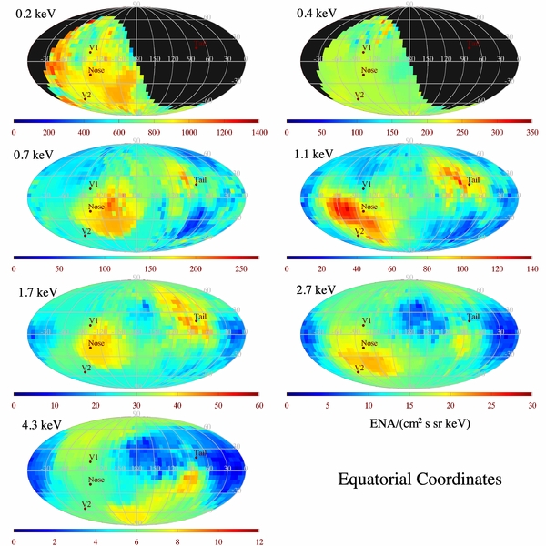
Figure 6. GDF in equatorial coordinates using the first 5 years of IBEX data.
Download figure:
Standard image High-resolution image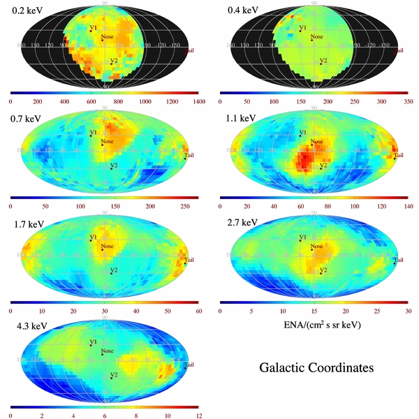
Figure 7. GDF in galactic coordinates using the first 5 years of IBEX data.
Download figure:
Standard image High-resolution imageWe fit the GDF as a function of energy to determine the spectral index, γ, where the differential flux in each pixel is approximated J∝Eγ and E is energy. The spectral index fitting uses a standard least squares method discussed by (Schwadron et al. 2011). Characterizing the differential flux using a spectral index in each pixel has been shown to be a reasonable approximation over most of the map. However, near the poles, we often observe broken ENA energy spectra (Dayeh et al. 2012). The spectral indices in the GDF are shown in Figure 8.
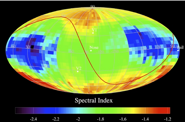
Figure 8. Spectral index of the GDF (the GDF is approximated J∝Eγ, where γ is the spectral index and E is energy) in each pixel. Note that we include both IBEX-Lo and IBEX-Hi data. Because IBEX-Lo data includes only regions centered on the heliosphere nose, we observe a break in the spectral index intensity at −30° and 180°.
Download figure:
Standard image High-resolution imageWe have calculated the pressure of plasma protons forming ENAs integrated over LOS where they are formed:
The limits of integration extend over the range of energies for which we have direct observational information from ENAs. The ENA flux is jENA(E) at energy E with corresponding particle speed v. This "LOS-integrated pressure" is calculated in the inertial reference frame (Figure 9). Note that in Figure 8 and in the top panel of Figure 9, we include both IBEX-Lo and IBEX-Hi data. Because IBEX-Lo data includes only regions centered on the heliosphere nose (defined by the upwind direction of the interstellar He flow), we observe a break in intensity at ecliptic longitudes of −30° and 180°.
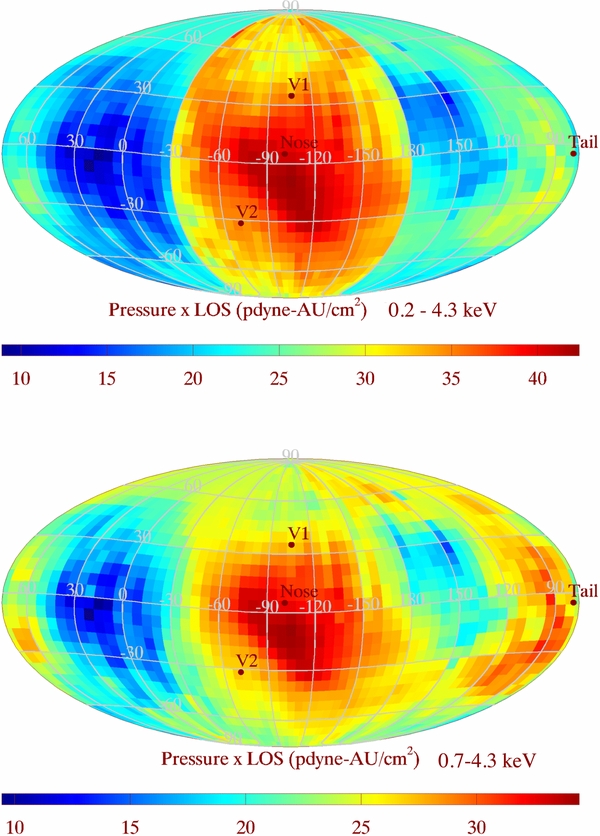
Figure 9. Pressure of plasma protons that form observed ENAs integrated over line-of-sight (LOS) as observed by IBEX and referenced to the inertial frame (see Equation (1)). The top panel includes both the IBEX-Lo measurements at 0.2 and 0.4 keV, and IBEX-Hi measurements from 0.7 to 4.3 keV. Because IBEX-Lo data includes only regions centered on the nose, we observe a break in intensity at −30° and 180°. The bottom panel includes only measurements from IBEX-Hi from 0.7 to 4.3 keV.
Download figure:
Standard image High-resolution imageFigure 8 reveals what has been pointed out in the first published maps (McComas et al. 2009a; Schwadron et al. 2009a; Fuselier et al. 2009a; Funsten et al. 2009b): the spectrum tends to harden at the poles and is softest near the tail. Originally, these trends were thought to be a property of both the ribbon and the GDF. However, subsequent work (Schwadron et al. 2011) where the GDF was studied separately showed that this property of the spectrum is driven by the GDF, even in the regions where the ribbon is observed. Understanding the detailed relationship between the energy spectrum and the varying global properties of the heliosheath remains an issue that has been studied only marginally using sophisticated modeling and theory. Recent work (e.g., Desai et al. 2014; Fuselier et al. 2014) has demonstrated both the ability of models to reproduce observations in the Voyager 1 direction and the direct extension of IBEX spectra into the much higher energies observed in situ by Voyager 1.
The GDF LOS-integrated pressure has a pronounced asymmetric enhancement near the nose (Figure 9). The asymmetric enhancement is shifted to the south and, near the ecliptic, the enhancement is shifted to the port direction (starboard and port are nautical terms detailed by McComas et al. 2013b).
Figure 10 shows the GDF centered on the interstellar downwind direction. We observe a clear signature of the tail along with the asymmetric lobes of ENA flux depletions (McComas et al. 2013b). Figure 11 shows the spectral indices of the GDF (top panel) and the LOS-integrated pressure (bottom panel) centered on the downwind direction. There is a LOS-integrated pressure enhancement shifted ∼10° to the starboard direction, yet the spectral index remains similar throughout the tail region including the side-lobes where the ENA flux is depleted. The softer spectrum near the tail region and in the lobes is likely due to the slower solar wind that, on average, emanates from the Sun in these regions (McComas et al. 2013b). The enhanced LOS-integrated pressure near the core of the tail is likely the result of the larger LOS that develops along the exhaust of heliosheath plasma. This suggests further that the large difference between the two tail lobes (i.e., the larger ENA flux depletion in port lobe) is driven by physical asymmetry of the lobes.
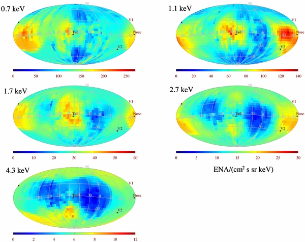
Figure 10. GDF shown with the projection looking down the heliospheric tail.
Download figure:
Standard image High-resolution image
Figure 11. Spectral indices of the GDF (top panel) and the pressure integrated along line-of-sight (bottom panel). The enhancement observed in both panels in the range of ecliptic longitudes from −30° to −180° is due to inclusion of IBEX-Lo data in this region. Note that the LOS-integrated pressure is in the heliospheric frame, not that of the plasma.
Download figure:
Standard image High-resolution imageBased on the LOS-integrated pressure (Figure 9) and the spectral index map (Figure 11), we define the following structures ordered by ecliptic longitude:
- 1.the nose region of pressure enhancement between ecliptic longitudes 160° and 320°,
- 2.the center tail region between ecliptic longitudes 50° and 130°,
- 3.the port lobe region between ecliptic longitudes −30° and 50°,
- 4.the starboard lobe region between ecliptic longitudes 130° and 180°.
The definition of these regions becomes useful primarily in identifying relationships between the longitudinal variation of the ribbon and the GDF.
Figure 12 (top) plots the total differential flux (no ribbon separation has been applied) of ENAs as a function of ribbon latitude in the frame of reference with a polar axis at the ribbon center. The normalized differential flux (we have multiplied each latitudinal distribution by a constant to normalize the maximum to 1.0) of the separated ribbon in this frame (bottom panel) allows direct comparison of the ribbon width and ribbon center as a function of energy. We observe broadening of the ribbon at higher energies (2.7 and 4.3 keV) and also at lower energies (0.2 and 0.4 keV). The ribbon appears most narrow at energies of 0.7 and 1.1 keV, which are energies associated with characteristic slow solar wind speeds of 370 and 460 km s−1, respectively.

Figure 12. Average differential flux (top panel) of ENAs as a function of latitude in the frame of reference centered on the ribbon, where the ribbon center is located at ribbon latitude +90°. The bottom panel is the normalized ribbon flux as a function of ribbon latitude.
Download figure:
Standard image High-resolution imageFigures 13 and 14 show the general characteristics of the ribbon. Shown in Figure 13 is the ecliptic latitude and ecliptic longitude of the ribbon as a function of the ribbon longitude in the rotated frame. This figure highlights the remarkable organization of the ribbon that is consistent across all energies observed. Shown in Figure 14 is the latitude of the ribbon peak in the rotated reference frame (top panels) and the FWHM (bottom panels) of the ribbon. The panel columns organized according to energy. General ordering of ribbon characteristics as a function of ecliptic longitude reveals the effects of heliosheath structure on the ribbon.
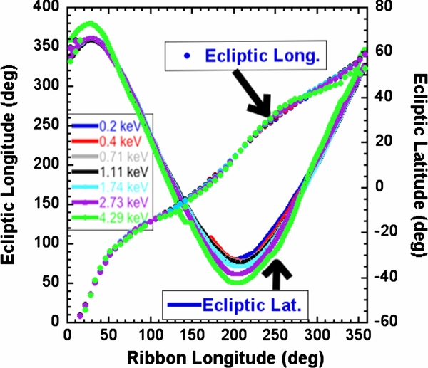
Figure 13. Ecliptic latitude and longitude of the ribbon (top) shown as a function of the ribbon longitude in the rotated frame where the ribbon center lies at ribbon latitude +90°. Different colors correspond to energies from 0.2 keV (blue) to 4.3 keV (green).
Download figure:
Standard image High-resolution image
Figure 14. Latitude of the ribbon in the rotated frame (top panels) and the FWHM (bottom panels) shown as a function of ecliptic longitude. The three columns of panels are organized according to energy with 0.4 keV (red) on the left column; 0.7 keV (gray), 1.1 keV (black) and 1.7 keV (light blue) in the middle column; and 2.7 keV (green) and 4.29 keV (purple) on the right column. The 0.2 keV data is not included due to its large uncertainties. In each panel we have included the ecliptic latitude of the ribbon (thin black curve) plotted according to labels on right-hand vertical axes. We also include the approximate boundaries between different regions of the heliosheath: nose, center tail, port and starboard lobes.
Download figure:
Standard image High-resolution imageThe ribbon latitude in the rotated reference frame reveals a number of organizing features. Figure 14(b), for example, at energies 0.7–1.7 keV shows that the ribbon appears almost at the same rotated latitude of ∼15° across the entire structure. If the ribbon were a great circle, it would appear at 0°. Instead the ribbon is shifted in latitude toward the ribbon center (the ribbon center in this rotated frame is at latitude +90°).
Consider the ribbon as a structure that lies along the surface where the radial direction (along the LOS) is perpendicular to the local interstellar magnetic field. In this case, the conical surface in Figure 15 represents the tangent surface containing the interstellar magnetic field at the location of the offset circle (the ribbon). Therefore the latitude of the ribbon may represent the deflection of the interstellar magnetic field due to draping at the location of the ribbon.

Figure 15. Geometrical construction of the ribbon latitude. A great circle exists at the intersection between a sphere of radius R (shown here) and a cylinder of the same radius. An offset circle with latitude λ with respect to the great circle exists at the intersection of a sphere of radius R and a right cone with a circular base of radius r = R/cos (λ) and height h = R/sin (λ). The center of the cone base is also at the center of the sphere. The latitude λ of the offset circle is also the half-angle of the cone. The center of the shifted circle is directed along the central axis of the cone. In the limit that λ → 0, the height of the right cone diverges and the conical surface converges to an infinite cylinder. In this case the offset circle converges to the great circle.
Download figure:
Standard image High-resolution imageIn both Panels (a) and (b) of Figure 14 for energies from 0.2–1.7 keV, we find an increase of ribbon latitude near the nose, suggesting increased draping in this region. In Figures 14(d) and (e), we observe a characteristic broadening of the ribbon near the nose that appears coincident with the increase in ribbon latitude. One interpretation is that this broadening may be the result of the changing deflection due to different amounts of draping along the LOS.
In Panels (c) and (f) of Figure 14 at 2.7 and 4.3 keV energies, we find broadening near the nose, but the ribbon latitude increases in an asymmetric manner. In particular, the ribbon latitude appears to increase only in the port side of the nose. Since the ribbon center is on the starboard side of the nose, the asymmetry may reflect interaction between the ribbon and the interstellar flow.
At or near ∼120°, we observe a decrease in ribbon latitude and a decrease in the ribbon width. Note that this ecliptic longitude is near both the tail and the region where the ribbon crosses the equator in the ecliptic (the ecliptic latitude of the ribbon is near 0°). The decrease in ribbon latitude indicates that the structure changes into something closer to a great circle. This shift and the decrease in ribbon width are both indicators that the ribbon is formed in a region where the interstellar field is closer to a planar structure in the asymptotic limit of no draping. The reduction of the ribbon width may also signify the departure from draping and return to an ordered planar structure along the LOS. These are characteristics that may naturally exist far from the Sun in the tail region.
3. DISCUSSION
In this section, we discuss implications of the separated maps of the ribbon and GDF. The discussion is organized first in terms of implications of the GDF for the heliospheric tail and lobes (Section 3.1) and for the region near the nose (Section 3.2). The considerations in these two first subsections are used to develop a basic picture for the global ecliptic structure of the heliosphere (Section 3.3). We then discuss implications of the separated ribbon maps for the source of the ribbon (Section 3.4).
3.1. Heliospheric Tail and Lobes
(McComas et al. 2012, 2013b) demonstrated for the first time based on the first three years of IBEX data the existence of a heliospheric tail centered close (within 15°) to the downwind direction. The spectral index of the energy spectrum is γ ≈ −2.3. (Figure 11, top) and is roughly uniform throughout the tail region. However, the pressure integrated across LOS (Figure 11, bottom) seems to peak slightly south of the ecliptic (∼ − 10° ecliptic latitude) at an ecliptic longitude of ∼90°, about 10° from the downwind direction (79° ecliptic longitude). Centered at about 15° ecliptic longitude we observe a deep reduction in ENA flux in the port lobe and a shallower ENA flux reduction from 140° to 180° ecliptic longitude in the starboard lobe.
We consider the implications of the pressure integrated across LOS for global heliospheric structures near the tail and in the two lobes. Recall that the LOS-integrated pressure as shown in Figure 11 is in the heliospheric frame, not that of the plasma. The formula for converting the LOS-integrated pressure to the plasma frame was developed by (Schwadron et al. 2011) and found to depend on the downstream flow speed and the spectral index.
(Schwadron et al. 2011) developed and applied a simple mass-loading model that provides necessary context for detailing the plasma environment of the tail, and thereby, interpreting the integrated LOS pressures in the GDF. The model based on (Isenberg 1987) applies conditions near 1 AU and integrates the solar wind plasma properties out through the heliosphere as new pickup ions created from interstellar neutral atoms mass-load the solar wind. The effect of mass-loading reduces the solar wind speed with increasing distance from the Sun. Here, we apply the mass loading model assuming a solar wind particle flux at 1 AU of 3.5 × 108 cm−2 s−1, a solar wind speed at 1 AU of 450 km s−1, and a neutral hydrogen density of 0.07 cm−3. These values are derived from solar wind conditions consistent with a period of time roughly 8 years ago, in the time frame of 2006. The 8 year delay time is associated with the time required for solar wind to move back into the heliotail (1.5 years to 150 AU in supersonic solar wind, 4 years for plasma to move an additional 100 AU in the subsonic inner heliosheath, and 2.5 years for ENAs to travel back to IBEX).
The pressure in the frame of reference moving with the plasma at radial speed uR is

where
are the internal plasma pressure and ram pressure, respectively. The limits of integration extend over the portion of the plasma distribution function (fp) for which we have direct observational information from ENAs. The distribution function of ENAs is fp, ENA(vp) = fp(vp)/[nHσ(Ep)LOS], where nH is the neutral H density, and σ(Ep) is the charge-exchange cross section at energy  . Here, the subscript p indicates the plasma frame. The velocity of a particle in the plasma frame, vp, is related to the velocity in the inertial (or observer) rest frame, vo, by the following relation,
  , where the unit radial vector is
  . The particle velocity is directed radially inward toward the observer so that
  . The observed differential flux, jo, ENA(Eo) = fo, ENA2Eo/m2. Incorporating these transformations, we express the internal and ram pressure as follows:
We use the mass loading model and the observed properties of ENA flux to derive a correction factor for the LOS-integrated stationary pressure shown in Figure 11. When analyzing the tail it is important to recognize that the plasma keeps flowing down-tail. The LOS in this case (near the tail) is the distance over which the primary plasma from the solar wind becomes neutralized through charge-exchange. The charge-exchange process merely transforms the originally hot solar wind plasma into a cooler and slower plasma dominated by interstellar atoms. (Schwadron et al. 2011) used the term cooling length to refer to this characteristic distance over which charge-exchange cools and slows the plasma. Because the material in the tail is not diverted or stagnated, the LOS-integrated internal pressure provides the basis for comparison to the mass-loading model.
Equation (5) determines the correction factor that multiplies the observed LOS-integrated stationary pressure to determine the internal LOS-integrated pressure. The correction factor depends on the spectral index (γ = −2.3) in the observed ENA spectrum and the plasma flow speed downtail. The mass loading model results in a downtail flow speed of uR ≈ 110 km s−1 for a wide-range of possible termination shock (TS) radii from 100 to 170 AU. Applying these values, we find that the correction factor is C = 2.42. Based on the results in Figure 11, this implies the Pinternal, tail · LOS ∼ 73 pdyne cm−2 AU in the core tail, Pinternal, port · LOS ∼ 36 pdyne cm−2 AU in the port lobe and Pinternal, star · LOS ∼ 48 pdyne cm−2 AU in the starboard lobe. Note that near the tail we have the benefit of observations down to 0.7 keV, but not all the way down to 0.2 keV. As a result, these LOS-integrated pressures are lower limits for the actual plasma pressures.
The internal pressure of the inner heliosheath plasma (beyond the TS) is shown in red (Figure 16) as a function of TS radius from the mass loading model. Given the internal pressure, and the values for the LOS-integrated internal pressures, we then solve for the LOS length as a function of TS radius near the tail (dark blue), in the port lobe (purple) and in the starboard lobe (light blue).
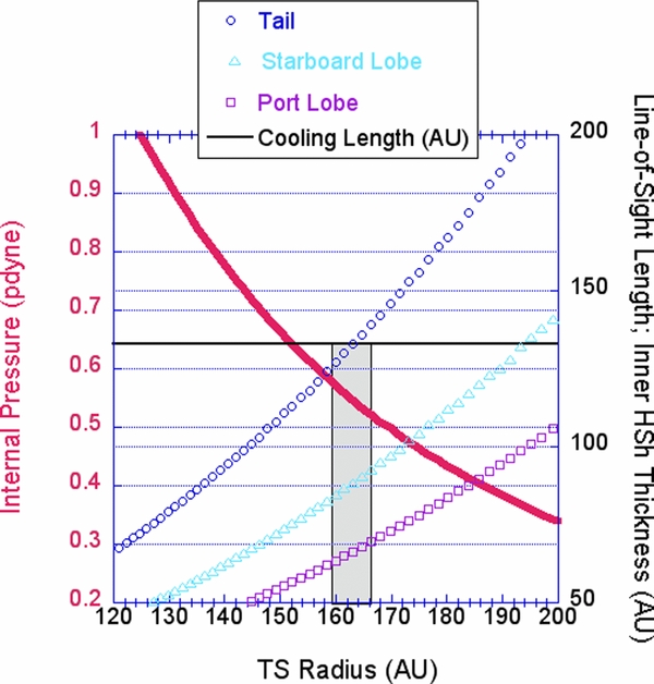
Figure 16. Internal pressure (red) of the heliosheath near the tail and the line-of-sight (LOS) length as a function of termination shock (TS) radius near the tail, in the starboard lobe and the port lobe. Also shown in black is the LOS limit, the cooling length from ENA charge-exchange. The limiting LOS length becomes large in the tail, and likely approaches the limiting value in the heliotail. This in turn sets a limit of ∼163 AU for the TS radius, and a minimum inner heliosheath thickness of 133 AU near the tail at 0.7 keV. The tail likely extends beyond the LOS limit, but our ability to observe the tail beyond this distance in ENAs becomes difficult. The reduction in ENA emissions near the port and starboard lobes suggests that their inner heliosheath thicknesses are less than 133 AU since the internal plasma pressure is roughly uniform across the tail region.
Download figure:
Standard image High-resolution imageThe cooling length, given by
sets a maximum for the possible LOS-length. The cooling length is shown as a function of energy in Figure 17. Based on the spectral index, the pressure integrated over LOS is dominated by the lowest energies observed (0.7 keV near the tail). This suggests a limiting LOS of 133 AU near the tail. Based on this constraint and the results shown in Figure 16, we estimate a TS radius near the tail of ∼163 AU.
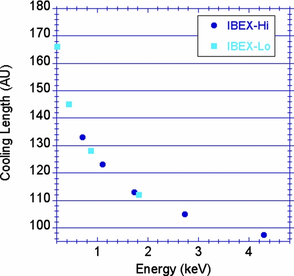
Figure 17. Cooling length across the inner heliosheath over the upper energy steps of IBEX-Lo (0.21, 0.44, 0.87 and 1.82 keV) and those of IBEX-Hi (0.71, 1.11, 1.74, 2.73 and 4.29 keV). The cooling length refers to the distance over which the plasma of the inner heliosheath near the tail cools substantially through charge-exchange.
Download figure:
Standard image High-resolution imageThe lower ENA emissions and LOS-integrated pressures in the port and starboard lobes suggest that the inner heliosheath thickness (dHsh) is reduced in these regions. Assuming that the internal pressure is roughly uniform across the tail and in the lobes, we find dHsh ∼ 66 AU in the port lobe and dHsh ∼ 89 AU in the starboard lobe.
In addition to LOS lengths, the internal pressure in the tail region provides an important measurement. We find Pinternal, tail ∼ 0.55 pdyne cm−2, which is slightly higher (by a factor of 1.5) than the magnetic pressure induced by a 3 μG magnetic field. A small 23% compression of the LISM magnetic field would induce a comparable internal pressure in the tail.
One of the consequences of the reduction of cooling length with increasing energy (Figure 17) is that the tail feature should fade with increasing energy. Figure 11 shows clearly that the tail feature fades for energies greater than 1.7 keV. At these energies, the cooling length decreases to less than 100 AU and approaches the 89 AU inner sheath thickness in the starboard lobe. The consistency of the length-scales validates the developing picture of the tail region.
3.2. Heliospheric Nose
We observe a LOS-integrated stationary pressure of the GDF (see Figure 9) near the nose given by ∼42 pdyne AU cm−2. At the location of Voyager 1 and Voyager 2, this LOS-integrated pressure is ∼33 pdyne AU cm−2. For analysis near the location of V1, we apply the mass loading model assuming a 1 AU solar wind particle flux of 3 × 108 cm−2 s−1, a solar wind speed at 1 AU of 400 km s−1, and a neutral density of 0.08 cm−3. These values are derived from solar wind conditions consistent with a period of time roughly 4 years ago (in the time frame of 2010). The shorter transit time delay near the nose is due to the smaller distance of travel of solar wind ions from the Sun into the inner heliosheath. The slight enhancement of the neutral density compared to that in the tail region is due to reduced charge-exchange loss of neutrals since the path history of neutrals intersects a thin portion of the heliosheath prior to arrival near the nose.
The downstream plasma speed from the mass loading model near the nose is ∼100 km s−1 for a range of TS radii from 100 to 200 AU. Given a spectral index in the differential energy flux of γ = −1.7, we find that the correction factor is C = 2, which multiplies the observed stationary LOS-integrated pressure (Figure 9) to deduce the LOS-integrated internal pressure, as discussed previously. Based on the results in Figure 9, this implies that Pinternal, V1 · LOS ∼ 66 pdyne AU cm−2.
The trends in solar wind pressure and particle flux appear to be relatively stable over the five-year period for which maps were analyzed (McComas et al. 2013a), which implies that the distance to the termination shock should also remain roughly constant. When compared to the 2005 time frame when Voyager 1 crossed the termination shock, and adding about a year for transit time, the 1 AU solar wind dynamic pressure appears to be about 15% larger than in the 2009-2014 period during which IBEX observations were made. Given the 1/r2 decrease in solar wind pressure, the 1 AU observations suggest that the termination shock should have moved in to ∼87 AU during the 2009-2014 time period (for comparison, see Webber & Intriligator 2011). Assuming a TS radius of 87 AU, the mass loading model yields a downstream internal pressure of 1.7 pdyne cm−2. Dividing this pressure into Pinternal, nose · LOS, we find a LOS ∼ 40 AU, which would suggest a heliopause near 127 AU. This estimate is somewhat larger the latest results from Voyager 1 indicating that it has moved into a region that is close to interstellar plasma at ∼121 AU (Gurnett et al. 2013).
Note that our calculation assumes a stationary termination shock and heliopause. In order to consider potential implications of time-dependent changes in the sheath, we re-ran the separation of the ribbon from the GDF for the year 5 maps (in 2013). This time-period is roughly consistent with the time period of the Voyager 1 121 AU crossing when correcting for solar wind transit time. Figure 18 shows the resulting LOS integrated pressure. When compared to the LOS-integrated pressure over the full five years of data (Figure 9), we observe the significant (∼19%) reduction of LOS-integrated pressure near the nose. Since the solar wind properties appear to be comparably stable over this time frame (2009–2014), the reduction in LOS-integrated pressure appears to be associated with inward motion of the heliopause and therefore a reduction in the LOS. Specifically, since the LOS-integrated pressure is reduced by ∼19%, we find a LOS of ∼32 AU. Given a TS at 87 AU, this would suggest a heliopause crossing at 119 AU. This is only 2 AU smaller than the distance for the actual Voyager 1 crossing.
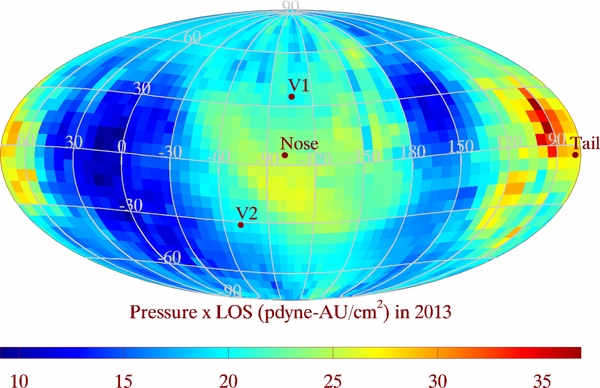
Figure 18. Pressure integrated along line-of-sight (LOS) as observed by IBEX in the year 5 maps (2013). The plot includes IBEX-Hi measurements from 0.7 to 4.3 keV.
Download figure:
Standard image High-resolution imageOne result is particularly interesting when Figure 18 is compared with Figure 9. While the LOS-integrated pressure near the nose drops, the tailward LOS-integrated pressure remains comparatively stable. Over the period from 2010 to 2014, we observe a fairly stable solar wind ram pressure, suggesting that the drop in LOS-integrated pressure near the nose is due to a more significant decrease in the LOS as compared to the plasma pressure across the nose region.
The ram pressure in solar wind was higher prior to 2010 than it was in the period from 2010 to 2014. This suggests that the inner heliosheath near the nose underwent inward motion to adjust to changing solar wind conditions. This inward motion must have occurred first at the termination shock, which responds immediately to local changes in the upstream supersonic solar wind. There is inherent latency in the inner heliosheath, which responds globally to average changes in solar wind over multi-year timescales since it is a subsonic medium. The reduction in solar wind pressure from 2006 to 2010 would have caused a steady inward motion of the termination shock (e.g., Richardson & Wang 2011), and a several-year latency in the inward motion in the heliopause. Due to the stability in solar wind ram pressure from 2010-2014, we expect that the termination shock would have largely stopped moving inward, while the heliopause continued to move inward over this time frame. The heliopause likely moved inward over Voyager 1 during the crossing.
3.3. Global Ecliptic Structure of the Longitudinally Asymmetric Heliosphere
Based on our analysis in the previous two subsections, we form a rough picture (Figure 19) of the heliosphere (termination shock and heliopause boundary) near the ecliptic plane. The termination shock distances and LOS thicknesses near the nose, tail and in the lobes are interpolated to illustrate the global structure. The direction of the interstellar magnetic field is given by the center of the IBEX ribbon and is projected into the ecliptic plane. The draping configuration is illustrative. This figure is approximate and its accuracy will evolve as the sophistication of GDF analysis improves. We emphasize that the LOS distance to the heliopause near the tail is essentially the charge-exchange cooling length. It is likely that the tail extends beyond this soft boundary, which sets a rough maximum for the LOS distance in this region.

Figure 19. Based on the analysis of the GDF, we have compiled an approximate structure of the heliosphere projected into the ecliptic plane viewed here from heliographic north. The structure near the nose is derived from both IBEX and Voyager 1 observations. The structure derived near the tail and in the lobes are the result of analyzing the LOS-integrated pressure. The downtail LOS is limited by the cooling length. Therefore it is likely that the tail extends well beyond the dashed line. The wavy lines extending from the lobes show regions beyond the LOS sensitivity of IBEX and suggest outflow. The tail region and structure of heliosheath is asymmetric. The clearest signatures of asymmetry include the small starboard (∼10°) offset of the core tail from the interstellar downwind direction, and the deeper reduction in ENA emissions from the port lobe of the heliosphere.
Download figure:
Standard image High-resolution image
Results of modeling of the heliosheath near the nose (see Figure 7 in Pogorelov et al. 2011) also show pressure structure consistent with asymmetries in the GDF (e.g., Figure 9). Both the modeled magnetic and total pressure on the heliopause is at a maximum near the upwind direction, but to the south by ∼15° and to port by a similar angle. While the southward deflection of total pressure appears consistent with the GDF LOS-integrated pressure, the shift in the pressure to port is opposite to the starboard shift in pressure observed in the GDF. This difference may again be a reflection of the asymmetry in the LOS. There remains a need to utilize global models of the heliosphere in combination with maps of the GDF to develop a consistent global picture heliosheath thickness and TS radius.
3.4. The IBEX Ribbon
One of the principal results of our analysis is the characterization of detailed properties of the IBEX ribbon. We discuss implications of this characterization in terms of suggested models of the IBEX ribbon, as recently reviewed (McComas et al. 2014b).
3.4.1. Inner Heliosheath: ENAs from Shock Processed Ions
One of the scenarios suggested by (McComas et al. 2009a) involves the production of the Ribbon ENAs at or near the termination shock by shock-accelerated pickup ions. The concept has been developed further by (Fahr et al. 2011), (Siewert et al. 2012), (Siewert et al. 2013), and (Kucharek et al. 2013). A strength of the concept in light of observations in Figure 14 is the organization of ribbon characteristics in terms of the nose and tail of the heliosphere. Specifically, we observe the ribbon become wider near the nose, narrower near the tail, and the ribbon latitude deviates to higher latitudes near the nose suggesting a smaller radius of curvature of the surface on which ribbon exists. These features are all consistent with the ribbon near the termination shock, which is closer to the observer near the nose and further away near the tail.
A difficulty in this scenario is the prominence of the ribbon at lower energies (0.2 and 0.4 keV), clearly much lower than the supersonic solar wind and pickup ions. Moreover, the characteristics of broadening and the organization of the ribbon latitude in Figure 14 change significantly as a function of energy. This would suggest that the physical structure associated with the ribbon (if it is a physical structure) changes depending on the energy of the associated population of ribbon particles. In contrast, the termination shock is physical structure independent of energy, and presumably we would observe characteristics (ribbon latitude and ribbon width) that are similar at varying energies.
3.4.2. Inner Heliosheath: Plasma Stagnation Region
Another explanation for the ribbon is that it originates from a region of high plasma pressure formed in the inner heliosheath to balance the combined ram pressure of the LISM flow and the J × B force exerted by the draped magnetic field on the heliopause (McComas et al. 2009a, 2010). The scenario remains difficult to test since there are no detailed quantitative models for the mechanism. One clear inconsistency is apparent: the observed ribbon broadens at both low energies (0.2 and 0.4 keV) and at high energies (2.7 and 4.3 keV). This implies that the pressure is carried predominantly by particles with energies 0.7–1.73 keV near the center of the ribbon and by higher and lower energies on the outskirts of the ribbon. Some mechanism is therefore needed to select particles to carry the dominant pressure in different regions.
3.4.3. Magnetic Reconnection and Instabilities at the Heliopause
Magnetic reconnection and magnetohydrodynamic (MHD) instabilities are expected to occur at or near the heliopause (Fahr et al. 1986) and were suggested as possible explanations for the ribbon by (McComas et al. 2009a, 2010) and (Schwadron et al. 2011). Magnetic reconnection that leads to interstellar flux transfer events has been proposed to explain recent observations by Voyager 1 showing interstellar plasma density but a magnetic field orientation consistent with that of the inner heliosheath (Schwadron & McComas 2013a; Strumik et al. 2013, 2014). (Kivelson & Jia 2013) used MHD modeling of magnetic reconnection at the Jovian moon Ganymede as an analogy for the configuration near the heliopause. They argued that the IBEX ribbon may be produced by ions heated by reconnection in localized regions on the heliopause. As with the first of the ribbon scenarios (ENAs from shock processed ions), the fact that magnetic reconnection is confined near a surface, the heliopause, implies that the location of the ribbon should be spatially well-defined. The specific ordering of the ribbon latitude (Panels (a)–(c) of Figure 14) that changes significantly as a function of energy becomes very difficult to explain if the ribbon exists at fixed locations along a surface.
3.4.4. Outer Heliosheath Source: Secondary ENAs
One of the original ideas presented by (McComas et al. 2009a) is that ENAs result from a population of ions in the outer heliosheath supplied by the neutral solar wind. Solar wind protons, like all protons, undergo charge-exchange with neutral H atoms that they come into contact with. There is an ample supply of neutral H atoms from the interstellar medium that move slowly through the heliosphere, at ∼23 km s−1. After a charge-exchange collision with an interstellar H atom, a solar wind proton is converted into a neutral H atom and moves out into the heliosheath at the speed of the solar wind particle from which it was created. As the neutral solar wind atom moves into the outer heliosheath, it eventually undergoes another charge-exchange reaction due to a collision with an interstellar proton. The neutral H atom is converted into a relatively high energy (∼1–4 keV) pickup proton and begins gyrating about the local interstellar magnetic field. Gyration causes a ring-beam of newly born pickup protons. If scattering rates are very low and the ring-beam can remain stable over years, the particles in the pickup ring undergo additional charge-exchange reactions, becoming neutral atoms moving in straight lines from their points of origin. If the neutral solar wind atom moves at roughly a right angle with respect to the interstellar magnetic field (B · r ≈ 0), then the particles remains almost stationary with respect to the field line, undergoing almost pure gyration.
Recall that the ribbon appears to be exist in locations where B · r ≈ 0 (McComas et al. 2009a; Schwadron et al. 2009a). Here, r is the radial direction and B is the interstellar magnetic field. In a direction where the B · r ≈ 0 condition is satisfied, particles from the ring-beam would have essentially an equal probability of having a perpendicular velocity directed with any of the 2π azimuthal angles about the interstellar magnetic field. Therefore, a fraction of the ring-beam is directed back in the radial toward the IBEX observer. Therefore, a fraction of the neutralized atoms from the ring-beam can be observed by IBEX.
(Heerikhuisen et al. 2010) developed the first detailed quantitative model based on this concept and demonstrated good agreement with observations. However, the model is far from free of assumptions and (Florinski et al. 2010) discussed a significant potential issue with the long several year scattering time required to maintain the ring-beam stability. (Chalov et al. 2010) and (Zirnstein et al. 2013) have developed even more sophisticated models of the ribbon based on this mechanism and (Gamayunov et al. 2010) argue that there are possible interstellar turbulence spectra that could give rise to the needed several year ring-beam stability. The reader is directed to (McComas et al. 2014b) for a more detailed review of work on the mechanism.
(Schwadron & McComas 2013b) developed a variant on the secondary ENA concept. The source from neutral solar wind and populations in the inner heliosheath is the same as in the original secondary ENA model (McComas et al. 2009a); however, the physical mechanism by which the ribbon is formed is different. As opposed to developing a model based on a metastable pickup ring, (Schwadron & McComas 2013b) consider the ribbon as a region where enhanced scattering retains protons. Scattering rates are increased through self-generated magnetohydrodynamic waves via the unstable pickup ring distribution in regions where ions are picked up with a small velocity component parallel to the magnetic field (the parallel velocity component must be smaller than the local Alfvén speed) and a large velocity component perpendicular to the magnetic field. This condition is satisfied typically near the directions where B · r ≈ 0.
A second model involving spatial ion retention has been developed by (Isenberg 2014), but in this case the model has difficulty accounting for the magnitude of observed differential ENA fluxes in the ribbon. While the (Isenberg 2014) and the (Schwadron & McComas 2013b) models have many similarities, they make significantly different assumptions about the nature of wave-particle interactions in the retention region. Understanding the underlying physical mechanisms in the ion retention region is an area of active research that holds significant promise for explaining the ribbon's origin.
The original ring-beam model of secondary ENAs relies on an optical effect in which the pickup ring is observable only when the observer lies near the plane perpendicular to the interstellar magnetic field. In contrast, the (Schwadron & McComas 2013b) and (Isenberg 2014) models involve a spatial effect in which the ribbon predominantly exists near the surface where B · r ≈ 0. Despite this fundamental difference between the mechanisms, they result in organization about the surface perpendicular to the local interstellar magnetic field and have identical sources. As a result, both mechanisms yield very similar predictions and distinguishing between them remains a significant challenge.
We note several points of consistency between secondary solar wind models and our observations of the ribbon. First, a typical supersonic solar wind speed inside the termination shock of ∼450 km s−1 should create secondary ribbon ENAs of ∼1 keV. A faster supersonic speed of 750 km s−1 should generate ribbon ENAs of ∼2.9 keV. in other words, the typical range of supersonic solar wind speeds spans much of the energy range where the ribbon appears to most localized.
The ribbon also persists at lower energies than the supersonic solar wind (0.2 and 0.4 keV) and at higher energies as well (4.29 keV). The ribbon broadens at these energies particularly near the nose and becomes most strongly distorted (shifts to higher latitudes in the rotated ribbon frame near the nose and to lower latitudes near the tailward ecliptic crossing, Figure 14). As pointed out by (McComas et al. 2009a), the secondary solar wind populations that populate the ribbon should emanate not only from inside the termination shock, but also from the inner heliosheath. The characteristic solar wind speed of this secondary source should extend down to at least 100 km s−1, with associated energy of the ribbon extending down to ∼0.06 keV. Further, since the solar wind population beyond the termination is much hotter than the solar wind inside the termination shock, we expect significant broadening of the ribbon at these lower energies, as observed.
The distortion of the ribbon at these lower energies could be a result of the lower characteristic LOS, which would cause the lower energy ribbon to illuminate the deviation of the interstellar magnetic field near the heliopause. In other words, the lower energy ribbon may provide fundamental new information about the draping of the interstellar magnetic field near the heliopause. This is an important problem that needs to be considered in future modeling work.
At 4.29 keV, an energy above the typical supersonic solar wind speed, pickup ions and suprathermal ions provide an additional secondary component. Pickup ions inside the termination shock typically extend to twice the solar wind speed inside the termination shock. Therefore, at 4.3 keV, we expect a source from secondary pickup ions in 450 km s−1 solar wind, which is a very typical speed for solar wind inside the termination shock. The pickup ion population is inherently a hot population and therefore should lead to broadening of the ribbon.
There is likely a plethora of different populations that contribute at these higher energies (>3 keV). In particular, energetic particles from suprathermal tails in interaction regions and within the heliosheath contribute as secondary populations at these energies. These populations are all hot and therefore should lead to significant broadening of the ribbon.
The ribbon latitude in the rotated frame at 2.7 and 4.3 keV in Figure 14 shows asymmetric deflection. We observe a shift of the ribbon to higher ribbon latitudes on the port side of the nose. Since deflection to higher ribbon latitudes is consistent with a reduced radius of curvature of the heliopause, the asymmetric deflection near the nose suggests draping from the nose toward the port flank of the heliosphere, as illustrated in 19.
Recall that a shift to higher ribbon latitudes is observed across the entire nose region at lower energies. (Möbius et al. 2013) shows that the combination of a 1/r2 dependence of the neutral solar wind and extinction processes results in 50% of the material that makes up the ribbon coming from ∼50 AU from the heliopause at 1 keV. At 4 keV the distribution of material in the ribbon becomes more distributed radially and at this energy 50% of the material comes from ∼80 AU from the heliopause. The configuration of the interstellar magnetic field also changes significantly with distance from the heliopause. Excluding magnetic reconnection, the interstellar magnetic field must be transverse to the heliopause along the boundary. However, far from the heliopause, the interstellar magnetic field becomes essentially planar. Approaching the heliopause the interstellar magnetic field becomes increasingly warped, or draped, as it transitions from a planar structure to one entirely transverse.
There is a consistency then between the observed signatures of the deformation of the ribbon near the nose. At low energies (lower than 2.7 keV), the signature is that of draping across the heliopause. At 2.7 and 4.3 keV, the asymmetric nose-port draping may be a natural result of the transition between the field configuration close to the heliopause and the field structure further out in the interstellar medium.
One of the important features observed in Figure 14 is the narrowing of the ribbon near the tail where the ribbon crosses the ecliptic plane. At this location we also observe a shift to lower ribbon latitudes in the rotated frame. Both of these features are consistent with the ribbon being pushed farther from the observer and returning to a more ordered planar structure as it crosses the tail. At 0.7–1.7 keV these effects are relatively small. For example the ribbon latitude and width drop by ∼3°–5°. However, at 2.7 keV and 4.3 keV, these effects become extremely pronounced. This again seems to indicate that higher energies are far more reflective of the large-scale ordering of the interstellar magnetic field.
3.4.5. Outer Heliosheath Sources
(Grzedzielski et al. 2010) proposed the concept that ribbon ENAs are produced in the interface between the Local Interstellar Cloud (LIC) and the Local Bubble (LB). The hypothesis is unlike the scenarios originally put forward by (McComas et al. 2009a). Hot, tenuous plasma of the LB undergoes charge exchange with neutral hydrogen from the LIC to produce ENAs. (Grzedzielski et al. 2010) calculated intensity profiles for ∼1 keV ENAs from the edge of the LIC ranging from ∼250 to ∼1100 AU and pointed out the resemblance of the ribbon to emission shells observed in astrophysical contexts could favor this source.
In light of the new observations of the ribbon provided here, several potential issues arise. First, the fact that the ribbon extends down to 0.2 keV raises the question of whether extinction would squelch the source at these low energies. The second potential problem is similar to that previously mentioned in the case of the source at the termination shock or the heliopause. There is a well-defined interface where the ribbon should be produced and this raises problems in understanding why the ribbon latitude in the rotated frame should vary significantly with energy. We expect fixed structures such as the LIC–LB interface to generate a feature that exhibits a similar structure across different energies. The energy variability of the ribbon latitude appears to be a significant departure from the likeness to "emission shells" observed commonly in astrophysical contexts. Notwithstanding these questions, the challenge remains to develop a LIC–LB model that accounts for the detailed features in the observed ribbon.
More recently, (Fichtner et al. 2014) provided a new hypothesis that the ribbon is a consequence of inhomogeneities in the local interstellar medium. When propagating through the heliosphere, such a wave of hydrogen enhancement (the "H-wave") can lead to higher flux of ENAs and would also account for absorption features in the Lyα lines measured toward nearby stars. However, because the H-wave is well-defined physical structure, the variability with energy of ribbon latitude in the rotated frame again poses a challenge to the concept.
4. SUMMARY AND CONCLUSIONS
We have conducted the second analysis in which we have separated the IBEX ribbon from the GDF. With the benefit of 5 years of data from IBEX, we have resolved and analyzed full-sky maps for both the ribbon and GDF. We also now have the addition of ribbon separation involving IBEX-Lo data down to 0.2 keV. The more complete analysis reveals features that were not apparent in the first ribbon-separation analysis (Schwadron et al. 2011) yielding a wealth of new information about our global heliosphere:
- 1.Global asymmetry. An important result from the analysis is the existence of an asymmetry in the global heliosphere observed both in the thickness of the heliosheath near the tail and the offset of the tail. The heliosheath appears to be thinner on its port side, and the tail is shifted toward the starboard direction. Both effects suggest a pressure enhancement on the port side, possibly a manifestation of compression and draping of the magnetic field. This result and our understanding of heliospheric asymmetry are ripe for further work involving global heliospheric modeling.
- 2.Cooling-length limit for LOS. We have shown that the cooling-length limit for the LOS decreases with increasing energy. This is consistent with observations in Figure 5 showing that that tail signature erodes at energies greater than 1.7 keV where the cooling length becomes smaller than 100 AU.
- 3.Broadening of ribbon in relation to magnetic draping. We observe a general trend in the ribbon (Figure 14) showing its width broadens near the nose of the heliosphere. This suggests the importance of magnetic draping that distorts the interstellar magnetic field, moving the ribbon to higher latitudes in the frame centered on the ribbon (Figure 14, bottom panel). Conversely, near the tail the ribbon appears to be most narrow and is shifted to the lowest latitudes in the ribbon-centered reference frame, consistent with a slight elliptical elongation of the ribbon found by Funsten et al. (2013).
- 4.Time variability near the nose. We have also re-analyzed the properties near the nose of heliosphere based on the LOS-integrated pressure in ENAs observed there. Taking into account recent Voyager 1 observations, we develop a rough model of ENA emissions near the nose that demonstrates the importance of time variability in the heliosheath. In comparing the LOS-integrated pressures averaged over 5 years versus those in 2013, we find that the pressure in the inner heliosheath nose region has dropped significantly in 2013. Given the relative stability of the solar wind pressure from 2010 to 2014, our results suggest that the heliopause has been moving inward over this time frame, a latent response to the drop in solar wind pressure occurring from 2006 to 2010.
- 5.Examination of ribbon models. The separated maps of the IBEX ribbon have allowed careful examination of the ribbon models. Generally, the variability in the properties including the central location of the ribbon as a function of energy suggest that the ribbon does not exist at a well defined physical location or at an interface. This constraint poses a significant problem for a number of the proposed models. The ribbon also exists as separable structure down to 0.2 keV. However, at these low energies, the ribbon both broadens and exhibits considerable variability in location as a function of ecliptic longitude.
The key products of our analysis are separated maps of the IBEX ribbon and the GDF. These maps will be the subject of the next IBEX data release (release 8). Generally, we observe the ribbon in every energy step analyzed from 0.2 keV up through 4.29 keV involving both IBEX-Lo and IBEX-Hi data. The resulting maps of the ribbon and the GDF have fundamental implications for the structure of our global heliosphere, and the structure, source and energy dependence of the IBEX ribbon.
We are deeply indebted to all of the outstanding people who have made the IBEX mission possible. This work was carried out as a part of the IBEX project, with support from NASA's Explorer Program. J.S., M.B., and M.A.K. were supported by the Polish National Science Centre (grant 2012-06-M-ST9-00455).